CHAPTER 3 ALL PARTS: Business Statistics and Data Analytics Flashcards
Foundations of Data Analysis: Populations, Samples, and Analytics Frameworks
Data analytics structures raw data into actionable business insight through systematic models such as the SOAR model. The SOAR framework consists of four sequential stages: Specifying the business question, Obtaining the relevant data, Analyzing the data using statistical tools, and Reporting the results to drive decision-making. In the data analysis phase, establishing clear boundaries around data subjects is essential, which requires defining the population and the sample.
A population comprises every single item, individual, or transaction of interest that shares a specified set of common characteristics. Analyzing an entire population yields definitive measures called parameters. For example, conducting a comprehensive operational survey across every restaurant in a country, or evaluating every customer in Amazon's global database, provides true population parameters. However, evaluating entire populations is typically impractical, prohibitively expensive, time-consuming, and resource-intensive due to massive data volumes.
To overcome population constraints, analysts work with a sample, which is a representative subset selected directly from the target population. Metrics calculated from sample data are defined as statistics. For instance, rather than analyzing all Amazon shoppers nationwide, an analyst might select a sample of shoppers located in Tallahassee, Florida. The ultimate goal of working with sample statistics is to perform statistical inference—drawing sound conclusions and making generalizations about the unobserved characteristics of the overall population based on patterns observed within the sample.
Data analysis encompasses three progressive tiers of statistical work:
Descriptive Statistics: Summary measures that aggregate, organize, and describe the basic characteristics of a known data set (whether a sample or a full population).
Inferential Statistics: Advanced measures computed exclusively from sample data to draw conclusions, estimate parameters, and generalize findings to the broader population.
Hypothesis Testing: A structured decision-making procedure where analysts formulate proposed explanations or assertions regarding population parameters and test them using sample statistics to determine whether empirical evidence supports or contradicts the proposed business claims.
Sampling Methodologies and Data Reduction Techniques
Selecting an appropriate sampling technique is necessary to ensure that sample statistics accurately reflect population parameters without introducing structural distortion. There are four primary sampling methodologies used in business analytics:
Simple Random Sampling guarantees that every observation in the target population has an equal and independent probability of selection. This approach is optimal when the underlying population is relatively homogeneous and no specific subgroup requires dedicated representation. In software environments like Excel, simple random sampling can be executed using built-in functions such as to assign uniform random numbers between and to records, which are then sorted and selected, or by using the sampling module in the Data Analysis ToolPak.
Stratified Random Sampling is used when a population contains distinct, identifiable subgroups (strata) based on demographic, geographic, or functional attributes (such as academic majors across a university business college, including Finance, Accounting, Management Information Systems, Risk Management and Insurance, Sales, Management, and Real Estate). The process involves three steps: first, dividing the population into mutually exclusive strata; second, calculating the exact proportion of the total population represented by each stratum; and third, performing simple random sampling independently within each stratum to ensure that every subgroup is represented in the final sample in exact proportion to its presence in the population.
Cluster Sampling also begins by dividing the population into distinct subgroups (clusters), such as academic class standing (freshmen, sophomores, juniors, and seniors) or geographical zip codes. However, unlike stratified sampling—which samples a few individuals from every group—cluster sampling selects a few whole clusters and includes every single individual within those selected clusters while leaving unselected clusters entirely out of the sample. This approach reduces data collection costs when clusters naturally mirror the diversity of the broader population.
Convenience Sampling (also known as non-probability sampling) selects data points based on ease of access, low cost, or immediate availability rather than randomized selection. Examples include surveying nearby customers at a local pizza restaurant or polling students strictly within a single major. While convenience sampling saves time and budget constraints, it risks producing unrepresentative samples that cannot be generalized to the broader population. Convenience sampling is executed either by selecting an easily accessible subset of existing records or by distributing surveys and terminating data collection the moment a target sample size is reached.
When working with massive enterprise databases, analysts perform data reduction—the process of reducing large, complex data sets down to manageable sizes tailored for business projects. Data reduction isolates critical, abnormal, or strategically relevant records, thereby accelerating computational processing speed and decreasing analytical costs. Filtering is the standard data reduction technique, isolating records based on designated column criteria. In Excel, filtering is applied by navigating to Data > Sort & Filter > Filter and selecting criteria from column drop-down arrows (such as filtering nationwide sales data down to the state of Texas).
Sources of Bias in Analytics and Mitigation Strategies
Bias represents prejudice or systematic error in favor of or against a person, group, thing, or idea relative to another. Bias can enter at any stage of business analytics—during initial data collection, computational analysis, or final presentation of findings—and can occur intentionally (such as selectively presenting data to support a predetermined outcome) or unintentionally (resulting from flawed sampling procedures or misinterpreted data).
There are four distinct types of analytical bias:
Nonresponse Bias: Systematic distortion occurring when survey respondents differ meaningfully from non-respondents. This frequently occurs when surveys are overly long, poorly structured, or demand invasive personal information, prompting specific demographics to opt out. Nonresponse bias is mitigated by transparently communicating the survey's importance, assuring respondent anonymity, keeping instruments concise, and offering participation incentives such as gift cards or entry into prize drawings.
Selection Bias: Error occurring when an analyst systematically selects sample elements that favor a personal belief, hypothesis, or convenient demographic while excluding others. For example, relying exclusively on Tallahassee residents to draw conclusions about general consumer spending across Florida introduces selection bias because Tallahassee's population is heavily concentrated with college students whose income and spending habits differ significantly from working professionals in major metropolitan areas like Orlando, Jacksonville, or Miami. Selection bias is minimized using simple random or stratified sampling.
Confirmation Bias: The tendency of analysts to evaluate, interpret, and present data in ways that selectively validate pre-existing beliefs, hypotheses, or management preferences while ignoring, suppressing, or discounting contradictory evidence.
Outlier Bias: The disproportionate distortion of aggregate summary metrics (such as the arithmetic mean) caused by extreme, unrepresentative observations. Outliers should never be blindly discarded nor uncritically aggregated; instead, they must be isolated, thoroughly investigated, and reported with contextual explanations.
Variables, Data Types, and Probability Distributions
Variables capture operational metrics that fluctuate across time or subjects, such as monthly sales revenue or operational processing times. These variables generate numerical data that dictate which statistical distributions and analytical methods are valid.
Numerical data is categorized into two distinct types:
Continuous Data: Quantitative measurements that can take on any real numerical value along a continuum, including fractional and decimal values. Continuous data represents an infinite set of possible values between any two given observations. Examples include customer age, physical weight, monetary currency values (, ), process duration in days (such as order processing times spanning to days, to days, or to days), and student Grade Point Averages ( to ).
Discrete Data: Quantitative measurements restricted strictly to whole numbers (integers). Discrete data contains a finite set of values between any two observations. Examples include the number of daily inventory units, pending order counts, active delivery vehicles, or manufacturing plant locations. One cannot observe units of product or pending orders; discrete metrics must jump in integer increments.
A probability distribution is a statistical function that describes all possible values a variable can take and the relative likelihood of occurrence for each value across a sample or population:
Uniform Distribution: A continuous distribution represented by a rectangular shape, where every single outcome within a defined minimum and maximum boundary possesses an identical probability of occurrence (for example, when customer shopping duration between minutes and minutes is equally distributed).
Normal (Gaussian) Distribution: A continuous, symmetric, bell-shaped probability distribution where observations cluster tightly around the central mean, with frequency decreasing symmetrically as values move further into the outer tails.
Binomial Distribution: A discrete probability distribution applicable to scenarios involving a fixed number of independent trials where each trial yields only one of two binary outcomes (such as purchase versus no purchase, or default versus non-default). Binomial distributions can be symmetric or skewed based on outcome probabilities.
Poisson Distribution: A discrete probability distribution modeling the count of events occurring per defined unit of time or space (such as customer arrivals per hour or defects per square foot of material). It typically displays a low mean and strong rightward skewness.
Measures of Central Tendency and Data Distribution Shapes
Measures of central tendency describe the single central focal point around which a numerical data set clusters. The primary measures include the mean, median, and mode:
The arithmetic mean is the universal average, calculated by summing all observations and dividing by the total observation count (): The mean incorporates every observation in the data set, making it valuable yet highly susceptible to extreme outliers.
The median is the spatial midpoint of an ordered data set arranged from smallest to largest value. If the observation count is odd, the median is the exact center value; if is even, it is the average of the two middle values. The median is resistant to outliers.
The mode is the most frequently occurring value in a data set. A distribution can be unimodal (one mode), bimodal (two modes), or multimodal (more than two modes). The mode is the only measure of central tendency capable of summarizing non-numerical categorical data.
Evaluating the relative positions of the mean, median, and mode reveals the underlying shape, symmetry, and skewness of a distribution:
Symmetrical Distribution: A balanced distribution where the left and right halves are mirror images, yielding . A standard bell curve exemplifies perfect symmetry with a skewness coefficient of .
Right-Skewed (Positive Skewness): A distribution where the tail extends far toward higher values on the right side. High-value extreme outliers pull the mean upward, resulting in , while the mode remains at the left peak. Examples include difficult examinations (where most students score low, but a few high scores pull the average up) or wage distributions (where a few high earners drag the mean above the median).
Left-Skewed (Negative Skewness): A distribution where the tail extends far toward lower values on the left side. Low-value extreme outliers drag the mean downward, resulting in , while the mode stays near the higher end. An example is an easy examination where most students score high, but a few low scores pull the average down.
Kurtosis measures the tail thickness and peak sharpness of a probability distribution relative to a standard normal distribution (which has a theoretical kurtosis of , or an excess kurtosis of ):
Leptokurtic (Positive Excess Kurtosis): A distribution featuring a tall, sharp central peak with heavy, fat tails. Observations are tightly clustered near the mean, but extreme tail events occur with higher probability, indicating elevated volatility risk.
Mesokurtic: A standard normal distribution shape with excess kurtosis equal to
Platykurtic (Negative Excess Kurtosis): A distribution featuring a flatter peak and thin, light tails. Observations are dispersed broadly across a wide range without clustering heavily at the center.
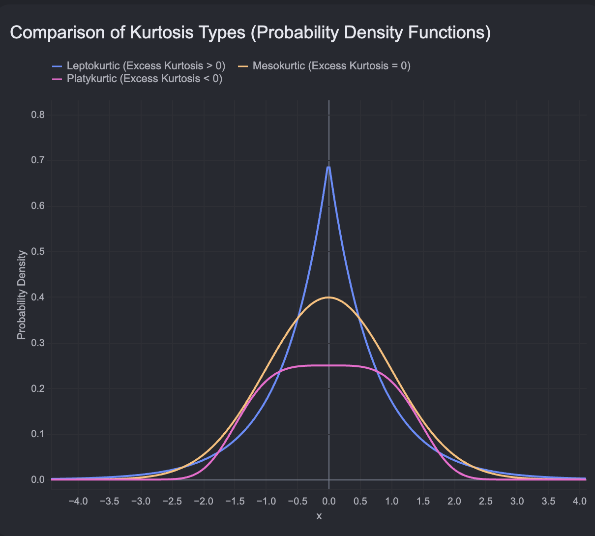
Measures of Dispersion and Standard Normal Distribution
Measures of dispersion quantify the degree of spread, variability, or scatter within a numerical data set:
The Range represents the total spread between extreme values: While simple to calculate, the range relies exclusively on extreme values and fails to describe how intermediate data points are distributed.
The Interquartile Range (IQR) measures the spread of the middle of observations, focusing on the distance between the first quartile (, the percentile) and the third quartile (, the percentile): Data is divided into four equal quartiles: (minimum to percentile), (the median, to percentile), ( to percentile), and ( percentile to maximum). By ignoring the upper and lower of data, the IQR eliminates outlier distortion.
Variance measures the mean squared deviation of individual data points from the arithmetic mean. Sample variance () divides by to provide an unbiased estimate of population variance (): Because variance is expressed in squared units, it is difficult to interpret directly in practical contexts.
The Standard Deviation is the positive square root of variance, restoring the measure of spread to the original measurement unit of the underlying data: In financial management, standard deviation serves as the foundational metric for asset volatility and risk.
For any perfectly normal continuous distribution, the Empirical Rule (68-95-99.7 Rule) governs the theoretical probability coverage of standard deviation bands centered around the mean ():
encompasses approximately of all observations.
encompasses approximately of all observations.
encompasses approximately of all observations, leaving only as potential extreme outliers.
For example, given a sample with a mean income of and a standard deviation of :
One standard deviation () spans () to (), containing of the population.
Two standard deviations () span to , containing of the population.
Three standard deviations () span to , containing of observations.
The Standard Normal Distribution is a theoretical standard reference distribution where the mean, median, and mode are equal to , and the standard deviation equals . Any individual observation from any normal distribution can be standardized into a Z-score, which indicates how many standard deviations lies above or below the mean: For example, given a population mean IQ of and a standard deviation of , an individual with an IQ of yields a Z-score of: This Z-score indicates intelligence four standard deviations above average.
Standard Error (SE) quantifies the expected variability or dispersion of sample means around the true population mean. Standard error shrinks as sample size () expands:
Summary Statistics Across Analytics Software Platforms
Modern enterprise analytics platforms generate descriptive statistics through automated routines. Standard formulas and tools vary across major software packages:
Excel Formulas:
Mean:
=AVERAGE(array)Median:
=MEDIAN(array)Mode:
=MODE.MULT(array)Skewness:
=SKEW(array)Range:
=MAX(array) - MIN(array)Interquartile Range:
=QUARTILE.EXC(array, 3) - QUARTILE.EXC(array, 1)Sample Standard Deviation:
=STDEV.S(array)Population Standard Deviation:
=STDEV.P(array)Sample Variance:
=VAR.S(array)Population Variance:
=VAR.P(array)
Excel Data Analysis ToolPak: Executing Data > Analysis > Data Analysis > Descriptive Statistics generates a unified statistical output table. For a sales data set comparing Sales Price and Cost, the ToolPak provides summary output across multiple parameters:
Mean Sales Price = ; Mean Cost =
Standard Error Sales Price = ; Standard Error Cost =
Median Sales Price = ; Median Cost =
Mode Sales Price = ; Mode Cost =
Standard Deviation Sales Price = ; Standard Deviation Cost =
Sample Variance Sales Price = ; Sample Variance Cost =
Kurtosis Sales Price = ; Kurtosis Cost =
Skewness Sales Price = ; Skewness Cost =
Range Sales Price = ; Range Cost =
Minimum Sales Price = ; Minimum Cost =
Maximum Sales Price = ; Maximum Cost =
Sum Sales Price = ; Sum Cost =
Count = records for both series
Interpreting these metrics reveals key product dynamics: because the mean exceeds the median for both attributes, both distributions exhibit positive rightward skewness driven by a small subset of high-priced products. Furthermore, Sales Price displays wider standard deviation and range relative to Cost, proving that while product cost influences retail pricing, additional commercial factors drive retail price dispersion.
Changing Default Aggregations in Business Intelligence Software:
Excel PivotTables: Right-click any value field >
Value Field Settings>Summarize Values Bytab > select Sum, Count, Average, Max, Min, Product, StdDev, or Var.Power BI: Select the field drop-down arrow within the visual settings pane > select Sum, Average, Minimum, Maximum, Count, Standard deviation, Variance, or Median.
Tableau: Right-click a measure pill > navigate to
Measure (Sum)> select Sum, Average, Median, Count, Minimum, Maximum, Percentile, Std. Dev., or Variance.
Visualizing Data Distributions: Histograms and Box Plots
Visualizing summary data provides intuitive insights into underlying distribution shapes, central tendencies, and dispersions.
A Frequency Distribution organizes raw quantitative observations into contiguous, non-overlapping numerical groupings called bins, classes, or intervals, displaying the count of observations falling within each bin.
A Histogram visually renders a frequency distribution using contiguous vertical bars whose heights reflect the observation frequency within each corresponding bin along the horizontal X-axis. Unlike standard bar charts—which display discrete categorical variables separated by gaps and can plot varying aggregations (such as sums or averages) on the Y-axis—histograms display continuous numerical data along the X-axis, feature no gaps between bars (unless a bin frequency is zero), and plot observation counts on the Y-axis.
A Box Plot (Box-and-Whisker Plot) displays data dispersion across quartiles:
Central Box: Spans the Interquartile Range (IQR) from ( percentile) to ( percentile), encompassing the middle of data.
Internal Indicators: A solid line drawn inside the central box marks the Median; an
Xsymbol marks the Mean.Whiskers: Lines extending outward from the central box to boundary fences indicating normal dispersion limits:
Outliers: Individual data points falling outside the boundary fences are plotted as isolated dots beyond the whisker boundaries.
Rotating a box plot degrees clockwise exposes distributional skewness: if the mean (X) sits above or to the right of the median line, the distribution is positively right-skewed; if the upper whisker extends far beyond the lower whisker, it reflects a long rightward tail.
Hypothesis Testing Foundations: Confidence Intervals and Formulations
Point estimates calculated from samples (such as a sample mean ) rarely match the true population parameter () exactly. To capture estimation uncertainty, analysts construct confidence intervals around point estimates.
A Confidence Interval defines a range of values constructed around a point estimate such that the true population parameter falls within the interval at a specified confidence level (such as , , or ):
The Margin of Error is calculated as a function of the chosen confidence level and the standard error of the sample. Expanding the sample size () compresses the standard error, producing narrower, more precise confidence intervals without sacrificing confidence coverage.
Hypothesis Testing is a formal statistical framework used to evaluate whether empirical sample evidence indicates a true, statistically significant effect or merely chance variation. The process follows four steps:
Step 1: Determine the Hypotheses
Null Hypothesis (): The default baseline assertion stating that no true relationship, effect, or difference exists between groups. Any observed sample difference is attributed strictly to random sampling variation.
Alternative Hypothesis ( or ): The statement tested against , asserting that a true, statistically significant relationship, effect, or difference exists in the population. If is rejected, is supported.
Directionality dictates test structure:
Two-Tailed Hypothesis Test: Evaluates whether a parameter differs in either direction (greater than or less than). For example, testing average hourly wages () across cities:
One-Tailed Hypothesis Test: Evaluates a specific directional difference. For example, testing whether Saturday sales exceed Sunday sales:
Step 2: Set the Significance Level (Alpha, ) The significance level () defines the threshold probability for rejecting the null hypothesis. It represents the maximum acceptable probability of committing a false positive error. Common baseline standards set ( risk), ( risk), or ( risk).
Step 3: Calculate the Test Statistic Using software like Excel (Data > Analysis > Data Analysis), analysts compute a sample test statistic (such as a -statistic or -statistic) and its corresponding -value.
Step 4: Reject or Fail to Reject the Null Hypothesis Using the -Value The -value indicates the probability of obtaining a sample statistic as extreme as, or more extreme than, the observed value if the null hypothesis were true. The decision rule is:
If : Reject . The evidence is statistically significant, supporting
If : Fail to reject . The evidence is insufficient to conclude a significant difference exists.
When interpreting software output, scientific notation like 2.23E-06 represents (or ), which is far below , prompting immediate rejection of
Decision Errors and Business Implications: Type I and Type II Errors
When testing hypotheses, sample statistics can lead to erroneous conclusions relative to true population realities. These outcomes are categorized into Type I and Type II errors.

Type I Error (Alpha Error / False Positive): Occurs when an analyst rejects the null hypothesis () based on sample results, when is actually true in the population. The probability of committing a Type I error equals the chosen significance level ().
Type II Error (Beta Error / False Negative): Occurs when an analyst fails to reject the null hypothesis () based on sample results, when the alternative hypothesis () is actually true in the population.
The real-world business implications of decision errors include:
Business Cost of Type I Error: Acting on something that is not true. In commercial operations, this means making capital investments based on false assumptions. For example, Google launching Google Glass in 2006–2008 represented a Type I error: leadership acted on the assumption that market demand was ready for consumer smart glasses, but consumer adoption failed, leading to product failure and lost capital.
Business Cost of Type II Error: Missing an opportunity that is actually true. This occurs when a firm fails to act due to conservative statistical conclusions. For example, stopping automated driving research because early data suggested low readiness—while competitors like Tesla successfully commercialized autonomous capabilities—represents a missed market opportunity.
Decision vs. Population Reality Matrix:
Decision: Reject (Conclude Different) | Reality: True (Population Same) Type I Error (False Positive)
Decision: Reject (Conclude Different) | Reality: True (Population Different) Correct Decision
Decision: Fail to Reject (Conclude Same) | Reality: True (Population Same) Correct Decision
Decision: Fail to Reject (Conclude Same) | Reality: True (Population Different) Type II Error (False Negative)
Analysts must avoid -value hacking—unethically testing multiple sample subsets or altering significance thresholds post-hoc to manipulate results until is achieved. Significance levels must be defined prior to executing statistical tests.
Statistical Significance Testing: t-Tests, ANOVA, and Chi-Square Tests
Selecting the correct statistical test depends on the underlying data types (numerical versus categorical) and the number of comparison groups:
Independent (Unrelated) Groups --Test: Compares the arithmetic means of two separate, non-overlapping numerical groups (such as comparing total spending of online shoppers versus in-store shoppers). In Excel, this is executed via t-Test: Two-Sample Assuming Unequal Variances when sample sizes or group variances differ.
Paired (Related) Groups --Test: Compares two dependent numerical measurements taken from the same subjects across two points in time (such as pre-test versus post-test scores for employees undergoing safety training). In Excel, this is executed via t-Test: Paired Two Sample for Means.
Analysis of Variance (ANOVA): Used to compare numerical means across three or more independent groups (such as comparing sales performance across website, mobile app, and in-store channels, or comparing long-term equity returns across SmallCap 600, MidCap 400, LargeCap 500, and S&P 500 indices). ANOVA calculates an -statistic to evaluate whether at least one group mean significantly differs from the others.
Chi-Square () Test of Independence: Used when working with categorical data rather than numerical measurements. It evaluates whether an observed categorical frequency distribution differs significantly from an expected theoretical distribution (such as evaluating payment method choices—credit card, debit card, cash, or mobile NFC tap—across customer segments like college students versus senior citizens).
Summary Comparison of Hypothesis Tests:
One-Sample --Test | Numerical Data | 1 Sample | Determines if sample mean significantly differs from a benchmark value.
Independent --Test | Numerical Data | 2 Unrelated Groups | Determines if sample means between two distinct groups significantly differ.
Paired --Test | Numerical Data | 2 Related Groups / Pre-Post | Determines if pre-test and post-test means from paired subjects significantly differ.
ANOVA Test | Numerical Data | 3 or More Unrelated Groups | Determines if significant mean differences exist across multiple groups.
Chi-Square Test | Categorical Data | 2 or More Groups | Compares observed versus expected categorical distributions.
Relationship Analysis: Correlation Analysis
Correlation analysis evaluates the direction and strength of the linear association between two continuous variables without assuming causation.
The Correlation Coefficient () quantifies linear association along a standardized scale bounded between and :
: Indicates no linear relationship between variables (for example, student height versus assignment completion rate yields , confirming no association).
: Indicates a perfect positive linear relationship where both variables increase proportionally (for example, student SAT scores versus college completion rate display strong positive correlation).
: Indicates a perfect negative linear relationship where one variable increases as the other decreases (for example, course failure counts versus college completion rate display a strong negative correlation of ).
In Excel, correlation matrices are generated via Data > Analysis > Data Analysis > Correlation. The resulting matrix yields values of along the diagonal, where each variable is correlated with itself.
Predictive Analytics: Simple and Multiple Linear Regression
Regression analysis builds upon correlation by modeling a functional relationship that uses independent input variables () to predict a continuous dependent output variable (): where:
= Dependent variable (the output metric being predicted).
= Independent variable(s) (the input metric(s) explaining variation in ).
= Slope coefficient (the rate of change in per unit change in ).
= -intercept (the baseline value of when ).
Simple Linear Regression incorporates one independent variable (). For example, modeling college completion rate () based on average institutional SAT score () produces the line of best fit: This indicates that for every -point increase in SAT average, college completion rate increases by approximately ().
Multiple Linear Regression incorporates two or more independent variables to explain the dependent variable. For example, adding Admission Rate () and Percent Pell Grant Recipients () alongside SAT Average () enhances the model's predictive power.
Key Regression Output Statistics:
Significance : Tests overall model validity. A Significance value below (such as
1.26E-285) proves the regression model provides significantly better predictive capability than a baseline intercept-only model.R-Square (): Coefficient of determination bounded between and . It measures the proportion of total variation in the dependent variable explained by the independent variable(s). An means the model explains of the variation in completion rates.
Adjusted R-Square: Used in multiple regression. Unlike standard —which automatically increases whenever a new variable is added regardless of quality—Adjusted penalizes unnecessary variables and increases only when an added variable genuinely improves model predictive power.
-Value of Explanatory Variable: Evaluates whether an individual independent variable is statistically significant. A confirms the variable is a meaningful predictor.
Causation Warning: Neither correlation nor regression proves cause-and-effect relationships. They measure mathematical association and predictive alignment, not causality.
Audience Interaction, Checkpoints, and Generative AI Tasks
Administrative Directives and Guidance:
Email Communication Standard: When emailing course instructors, students must explicitly include their assigned section number in the message text. Canvas direct messaging should be avoided.
Timezone Configuration Note: Canvas assignment deadlines were previously affected by Central Time versus Eastern Time system settings. System deadlines are aligned to Eastern Time.
Lecture Due Dates: Lecture materials have no formal due dates; posted dates serve as pacing guidelines for exam preparation.
Generative AI Practical Exercises:
Task 1: Use a Generative AI prompt to generate comparative corporate examples contrasting Stratified Sampling versus Cluster Sampling.
Task 2: Query Generative AI to identify real-world business case studies where sampling bias (such as selection bias or nonresponse bias) resulted in commercial product failures.
Knowledge Checkpoints:
Question 1: How does expanding sample size () impact standard error and confidence interval width? Answer: Expanding sample size () decreases the standard error (), which compresses the margin of error and yields a narrower, more precise confidence interval.
Question 2: Which statistical test is required to compare average transaction spending across three distinct retail formats (In-Store, Mobile App, and Web)? Answer: Analysis of Variance (ANOVA), because the comparison involves continuous numerical data across three independent groups.
Question 3: Given a calculated (
2.23E-06) and a significance threshold of , what is the statistical decision? Answer: Reject the null hypothesis (), because the is far below , indicating statistically significant evidence supporting the alternative hypothesis.
I initially said False because of the strict statistical definition of the Null Hypothesis () covered in Section 3.6 of your notes: 1. Null Hypothesis () always represents the baseline assumption of no effect or no difference (i.e., 'The drop in cancellation rate is NOT statistically significant'). 2. Alternative Hypothesis () represents the presence of an effect (i.e., 'The drop IS statistically significant'). Strictly speaking, the phrase 'they reject that the drop is statistically significant' misstates , because never asserts that a drop is statistically significant. However, the quiz author used informal phrasing intended to mean: 'Because , they reject , thereby concluding that the drop is statistically significant.' Since , rejecting to support statistical significance is the correct statistical decision.
The correct test to use is ANOVA (Analysis of Variance). ANOVA is used to compare continuous numerical means across or more independent groups (in this case, comparing average sales across the Loyal, New, and Occasional customer segments).