Week 3
t-Tests
Assess whether two means are statisically different
3 types:
One-sample t-tests compare a sample mean to a single value
e.g., comparing a sample to a known (or hypothesized) population mean
Independent-sample t-tests compare the means of two independent groups
Between-subjects designs
Paired-sample t-tests compare the means of two non-independent groups
Within-subjects designs
Depend on the Central Limit Theorem (CLT)
Central Limit Theorem (CLT)
If you repeatedly, randomly sample from a popualtion with mean μ, then the distribution of the sample means will be centered on μ and approximately normally distributed
The standard deviation of the sampling distribution will depend on N
t Distributions
The CLT lets us characterize a series of t Distributions with known characteristics (mean = μ; standard deviation that depends on N)
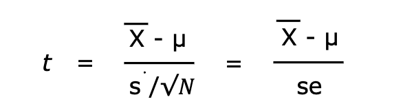
With a known N and a known x̄, we can calculate how far away Xis from the center of the relevant t distribution
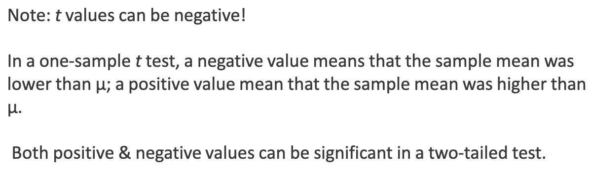
This yields a t value
Under the assumption that our sample(s) really do come from a distribution centered on μ, more extreme t values are less likely
Functionally this is a test of H0!
When there’s less than a 5% chance of obtaining our observed t value, we conclude that our sample(s) probably aren’t taken from a distribution cnetered on μ - that is the means differ
Note: with α = .05, our cut-off is a 2.5% likelihood in each tail (5% in total – this is a “two-tailed” test)
If our t value is more extreme than the “critical t values” at these cut-off points, then we reject H0
We’ll also get a p value that tells us exactly how likely our t value was under H0
One-Sample t-Tests
Compare a sample mean to a single value
Does the mean IQ of UIowa undergraduates differ from 100?
Do pigeons’ test scores differ from chance (50%)?
t-Tests are parametric, meaning that they rest on certain assumptions
(necessary to construct the underlying t distribution)
We have to check these assumptions before we run the t-Test
Steps for a One-Sample t-Test
Check the assumptions
The DV must be continuous
The observation must be independent
This is more about study design; not something we’ll test
The DV must be (approximately) normal
We’ll test for significant depatures of normality using a “Shapiro-Wilk” test
Calculate the t and p values
Report in standardized format
The sample mean[did / did not] significantly differ from [hypothesized value], t(df) = [], p = []
Where df (degrees of freedom) = N - 1
Assumptions of One-Sample t-Tests
If the assumptions are met, then we can run the t-Test
If the assumptions aren’t met, then we can’t run the t-test
Move to “non-parametric” stats, which are (a bit) more complicated but require fewer assumptions
We won’t deal with non-paraetric stats in this course