Reinforcement Learning
Reinforcement Learning:
receive feedback in the form of rewards
agent utility is defined by the reward function
must (learn to) act so as to maximize expected rewards
still assume MDP:
a set of states s ∈ S
a set of actions (per state) A
a model T(s, a, s’)
a reward function R(s, a, s’)
still looking for a policy π
now we don’t know T or R
therefore - experiement!
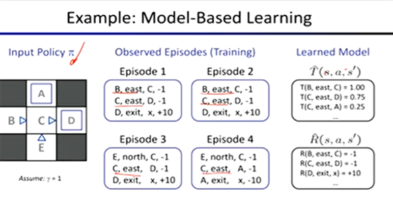
Model-Based Learning
learn an approximate model based on experiences
learn empirical MDP model
count outcomes s’ for each s, a
normalize to give estimate or T(s, a, s’)
discover each R(s, a, s’) when we experience (s, a, s’)
solve the learned MDP
Model-Free IL
Passive Reinforcement Learning:
policy evaluation
input: fixed policy π(s)
don’t know transitions or rewards
goal: learn state values
learner is “along for the ride”
no choice about what actions to take
just execute the policy and learn from it
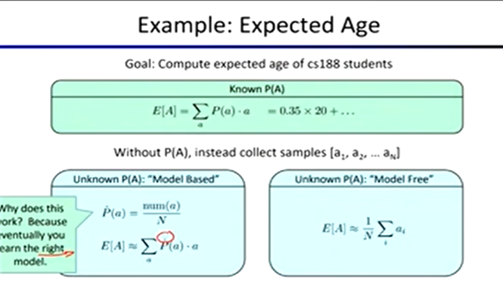
Direct Evaluation:
compute values for each state under π
average together observed sample values
ex A. output values:
A: -10, B: 8, C: [[(-1+10) + (-1+10) + (-1+10) + (-1 - 10)] / 4] = 4, D: 10, E: -2
Indirect Evaluation:
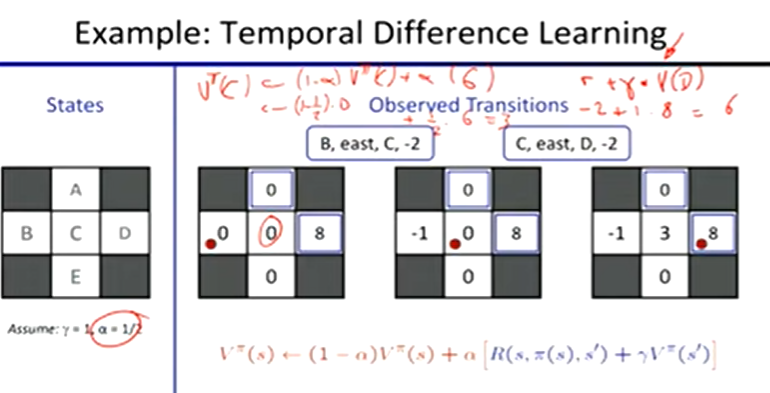
Temporal Difference Learning:
learn from every experience
update V(s) each time we experience a transition (s, a, s’, r)
policy still fixed, still doing evaluation
Sample of V(s)
sample = R(s, π(s), s’) + γVπ(s’)
Update to V(s)
Vπ(s) ← (1 - a)Vπ(s) + (a)sample
same update:
Vπ(s) ← Vπ(s) + a(sample - Vπ(s))
Exponential Moving Average
running interpolation update:
xbarn = (1-a) ⋅ xbarn - 1 + a ⋅ xn
Active Reinforcement Learning:
full reinforcement learning: optimal policies
don’t know transitions or rewards
choose the actions now
goal: learn the optimal policy / values
fundamental tradeoff: exploration vs. exploitation
Exploration:
How to explore? Random actions
every time step, flip a coin
with (small) probability ε, act randomly
with (large) probability 1-ε, act on current policy
when to explore?
random actions: explore a fixed amount
better: explore areas whose badness is not established yet, eventually top exploring
Exploration Function:
f(u, n) = u + k / n
Modified Q-Update:
Q(s, a) ← R(s, a, s’) + γ max f(Q(s’, a’), N(s’, a’))
Q-Value Iteration
find successive (depth-limited) values
start with V0(s) = 0
given Vk, calculate the depth k+1 values for all states
Vk+1(s) ← max ∑T(s, a, s’) [R(s, a, s’) + γVk(s’)]
but Q values are more useful so compute them instead:
Qk+1(s, a) ← ∑T(s, a, s’) [R(s, a, s’) + γ maxQk(s’, a’)]
Q-Learning
sample-based Q-value iteration
learn Q(s, a) values as you go
receive a sample
consider your old estimate
consider your new sample estimate
incorporate new into average
Off-policy learning
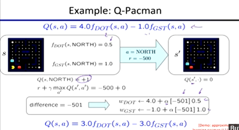
Approximate Q-Learning:
Generalizing across states:
learn about some small number of training states from experience
generalize that experience to new, similar situation
Feature-Based Representations:
describe a state using a vector of features (properties)
Q(s, a) = w1f1(s, a) + w2f2(s, a) + … + wnfn(s, a)
Transition = (s, a, r, s’)
difference = [r + γ max Q(s’, a’)] - Q(s, a)
Exact Q’s: Q(s, a) ← Q(s, a) + a[difference]
Approx Q’s: wi = wi + a[difference] fi(s, a)
Regret: measure of total mistake cost: difference between rewards and and optimal rewards
Policy Search:
often feature-based policies that work well aren’t the ones that approximate V / Q best
we should learn policies that maximize rewards, not the values that predict them
start with an ok solution then fine-tune by hill climbing on feature weights
simplest policy search:
start with initial linear value function or Q-functions
nudge each feature weight up and down and see if your policy is better than before