Topic 8
Assumptions of Repeated Measures ANOVA: Sphericity
Tests of within subjects effects always include several outputs based on whether or not sphericity is assumed – where sphericity has been violated, certain corrections for the degrees of freedom can be applied.
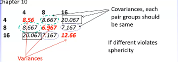
Sphericity regards whether the variances and covariances across pairs of RM groups are the same.
Therefore can only be tested with 3 or more levels to the RM factor
Compares the differences in co/variances differs between pairs of groups – where there is only two levels, only one set of differences is produced with nothing to compare to – therefore, sphericity is assumed (and p = 0)
A violation in sphericity bases bias in the F statistic – F becomes larger than it really is, which increases the risk of a type I error (seeing an effect when there isn’t one)
Usually apply the Huynh-Feldt adjustment which lowers the df and therefore makes it harder to find significance
df should always be rounded up to the nearest whole
Sphericity is tested using Mauchley’s test: if p < .05, sphericity has been violated
E.g., We have a main effect of distractors (4, 8, and 16 distractors)
Variance indicates how much the different levels of the IV distractor vary
The covariances indicate the unstandardised correlations between each level
Assumptions Common to All Designs: Normal Distribution, Homogeneity of Variance
Normality assesses how representative the mean of the DV is to the population of interest
Common to all ANOVAs
Because this is the overarching goal, in the event of a violation, it should always be asked: how does this violation influence the means and interpretation of analysis?
There are two main effects that can cause major problems to ANOVAs:
Floor effects: most people score very low / zero
Ceiling effects: most people score very high / the top score
These are problematic because:
If most people have the same score there is little in-group variance – the smaller the variance, the less variance there is to explain
The mean wont be representative – cannot account for scores lower/ higher that the floor or ceiling so these will be excluded from the mean and therefore make it nonrepresentative
In these instances, ANOVA cannot be conducted.
These problems cannot be fixed statistically, but there are some methodological considerations that can reduce the instance of floor and ceiling effects:
Pilot testing
Using reliable measures
Not collecting data on samples with low prevalence of the variable of interest (e.g., measuring dementia in 18 year olds; risky driving behaviours in women)
Homogeneity of variance examines whether the variance within each group is the same
Tested using Levene’s test: p < .001 indicates homogeneity of variance has been violated (because it is a conservative test)
If the distribution is nonnormal, violations may appear but won’t be a problem - should always compare group variances visually to confirm – look for distributions that may change the interpretation of the data
Where there are equal group numbers, violations can be dealt with - ANOVAs are robust to deviations from homogeneity of variance.
How to Test Assumptions of ANOVA
Example design: 2 (gender: men, women) x 2 (driving experience: not experienced, experienced) independent groups design where DV = risky driving behaviour
We need to investigate the distributions for each level of each factor.
Ideally, the mean and median will be pretty similar
The not experienced groups distributions looked pretty good. However, there were differences in variances between men and women (men had higher variances)
For the experienced groups, variances were very different for men and women (men much higher). The male group also displayed an extreme score.
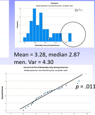
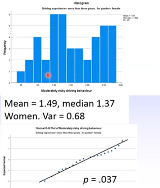
We would expect significant violations of normality for both of these distributions.
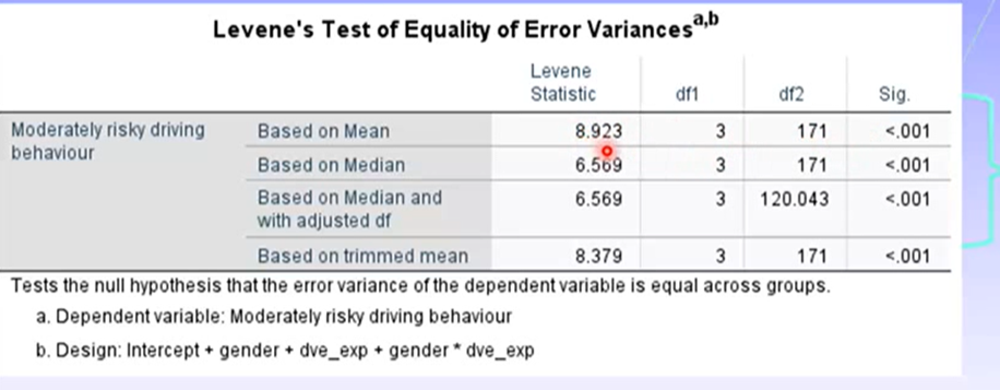
Levene’s test indicates all distributions sig violate homogeneity of variance, which makes sense because the variances were very different between men and women across all groups.
Ways to deal with this:
Could remove the extreme score, but we would have to do this for all groups
Need to be careful because trying to fix a problem in one group cn cause problems in the others
At this point it looks like the distributions are similar
Could be some extreme scores in male group
Variances across groups aren’t the same
A square root transformation may stabilise these variances, but must be applied on the whole of the DV
Square root transformation reduces the impacts of larger scores, therefore reducing variance.
Happens because there is less adjustment for smaller scores in the distribution (e.g., 100 = 20, 4 = 2, 1 = 1)
Does mean if there are any zero scores in the distribution we need to add one before applying the transformation
After applying this: distributions, normality, and Levene’s tests look a lot better. However, there has actually been no significant change in any of the analyses. Therefore, the violations of normality and homogeneity of variance has made no impact on the analysis – so the transformation should not be applied.
Always best to avoid transformations as they severely limit the interpretability of data (e.g., cannot report actual numbers, only that one group engages in DV more often)
The Influence of Unequal Numbers of Participants/ Unbalanced Designs in Factorial Designs
The ANOVA was designed for equal n in each group, which is why we try hard to not exclude any participants. However, sometimes an unequal n is inevitable (especially in field research). In these instances:
Ensure sums of squares III is used to generate any within subjects error terms – these treat each group as independent so they aren’t combined when generating an error term – this is the default in SPSS
Independent factorial designs experience the greatest issues with unequal n sizes.
Produce confounding or inaccurate results, especially for main effects: need to confirm means and SDs produced for main effects are the same as those in the descriptives generated prior to analysis
What Happens when there is a Small Number of Participants in One Group
Example: Analysis of gender – often gender is reported as male, female, or neither/other. Usually, there is far less people in the other/neither group.
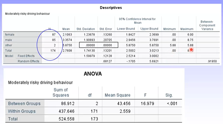
Can see the SD and SE for the other group is 0 – this is because they had the exact same score on the DV. ANOVA cannot be conducted accurately when there is such a small number of people in a group, and the SD = 0 – but SPSS will not know this automatically.
In most cases, this group should be excluded as the sample size distorts the analysis
Effect Sizes in ANOVA
Effect sizes are a family of statistical indices that give a measure of the strength and magnitude of the treatment effect
Are estimates based on an average of the whole dataset (either the mean, median, or correlation)
Why report effect sizes?
Indicates the magnitude of the treatment effect
Allow examination of the similarities and differences across studies using the effect sizes – useful in meta analyses
Don’t increase interpretability or practical meaningfulness of results – this is done by literature and theory
Types of Effect Sizes:
Unstandardised effect: used if they are meaningful on their own (e.g., years in school, raw test scores)
Standardised effect: used in the unstandardised effect is not directly interpretable or if we want to compare effect sizes across different units of measurement (e.g., Cohen’s d, beta, correlation)
Variance accounted for: the percentage of variance accounted for (e.g., R2, eta2, partial eta2)
Adjusted variance accounted for (e.g., adjusted R2, omega2, partial omega2)
Eta2: the proportion of variance in the DV accounted for by the main effect and interaction term – ranges 0-100%
(sum of squares treatment or group)/(total sum of squares)
Partial eta2: similar to eta2 but can add up across the various main effects and interactions to over 100%
Will be the same as eta where there is only 1 IV
(sum of squares of treatment)/(sum of squares treatment+sum of squares error)
Cohen’s d: estimates the distance between means in standard deviation units – can only be calculated if there are 2 groups in the IV
(Me-Mc)/SD
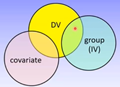
Analysis of Covariance: What is a Covariate
Covariates are variables that influence the DV but have no influence on the IV. They reduce the unexplained variance in the DV without sharing any variance with the IV, and therefore make it easier to find a significant effect of the IV
Should be measured prior to group allocation, then participants can be randomly allocated to groups
Must have a linear relationship with the DV in each level of the IV
Must have a completely independent effect of the DV to the IV
Example of this effect:
ANOVA ANCOVA
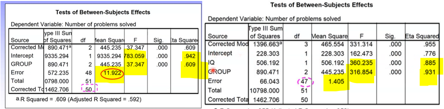
Can see:
Error term is much larger in ANOVA
F value and eta2 are much smaller
Significance doesn’t change
Conceptual Underpinnings of ANCOVA
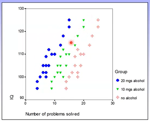
Example: IV = alcohol consumption, covariate = IQ, DV = problem solving ability
We know that alcohol consumption as a treatment condition is not at all related to IQ – therefore these variables are appropriate.
What if the covariate and IV are not independent?
Then we cannot use an ANCOVA
Any shared variance between the ‘covariate’ and IV is given entirely to the covariate and excluded from the analysis of the IV – making it harder to find a sig effect and therefore contradicting the purpose of an ANCOVA.
The error term in ANCOVA is calculated based on the difference between the raw score and the predicted value on the covariate (based on the regression line)
Group means for the covariate may vary slightly but should be nearly identical.
Should be the case if the covariate and IV are completely independent and participants are randomly allocated to groups
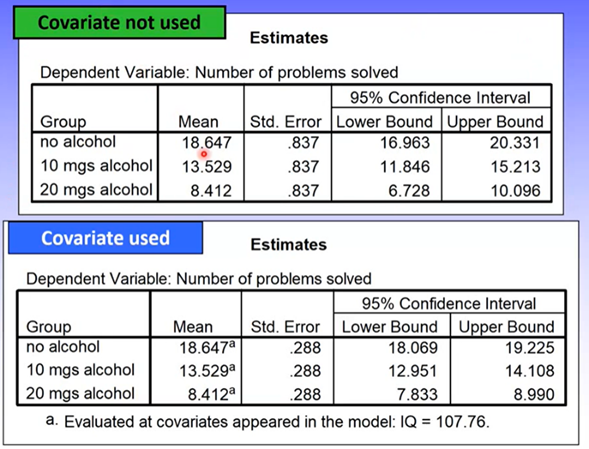
Can see the means are the same but standard errors / CIs have changed slightly (there’s increased precision)
Assumptions of ANOCOVA: Homogeneity of Regression
The main assumption of an ANCOVA is homogeneity of regression slopes: the same linear relationship between the covariate and DV should be found across all levels of the IV.
What this looks like:
Heterogenous regression slopes would look something like this:
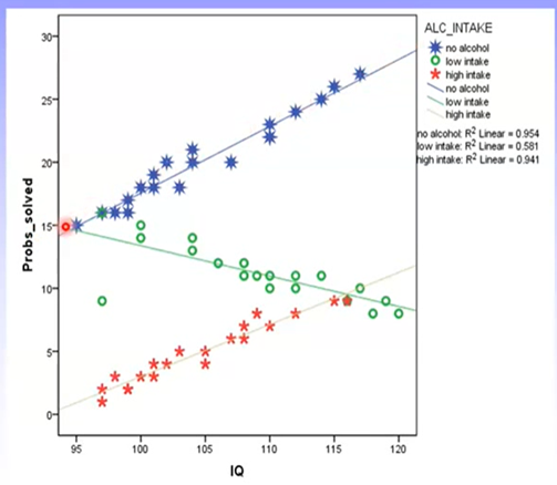
If homogeneity of regression is violated, ANCOVA cannot be conducted. This is because the covariate and IV are therefore not independent.
Other assumptions of ANCOVA:
Levels of the IV are normally distributed
Scores on the IV and covariate are independent
Measurements of the covariate are reliable
There is a linear relationship between the DV and covariate