Multiple Regression
Multiple & Hierarchical Regression
PS21310 - Quantitative Research Methods Lecture 5
Overview of Regression
Types of Regression
Simple Regression:
A linear approach for modelling the relationship between a dependent variable y and one or more explanatory variable denoted X.
Models the relationship between one dependent variable (DV) and one independent variable (IV).
Equation: Ŷi = (b0 + b1 * xi) + ei
Focuses on the direct linear relationship and allows for prediction based on one variable.
Multiple Regression:
Extends simple regression to multiple independent variables predicting one dependent variable.
Equation: Ŷi = (b0 + b1 * x1 + b2 * x2 +... + bi * xi) + ei
Enables understanding of how several variables simultaneously influence the DV.
Hierarchical Regression:
Allows for assessing the contribution of predictors sequentially.
Typically involves entering predictors in steps to observe how each addition affects the model and outcomes.
Key Components of Simple Regression
Ŷi: Predictive value of Y (expected value for the dependent variable).
b1: Regression coefficient indicating the quantity by which Ŷ increases for every one-unit increase in x (independent variable).
b0: Y-intercept (expected value of Y when independent variable x is 0).
xi: Value of the independent variable for a particular participant.
ei: Error term representing unexplained variance in the model's prediction.
Regression Assumptions
Key Assumptions:
Continuous dependent variable and normal distribution.
Linearity between the dependent variable (DV) and independent variables (IVs).
Normality of residuals (the difference between observed and predicted values must appear normally distributed).
Homoscedasticity (equal variance of residuals across values of IV).
Minimum sample size guidelines:
Green's (1991) rule: Minimum sample size = 50 + 8k, where k = number of predictors.
Additional Considerations:
If assumptions are not met, data transformation techniques (e.g., log-transforming) may be employed to improve model fit.
Multiple Regression Insights
Analysing Multiple Variables:
Explores contributions of various independent variables to the dependent variable.
Central questions addressed include:
How well do predictors estimate an outcome?
Which predictor is the strongest in terms of explanatory power?
Importance of each predictor while controlling for the effects of others.
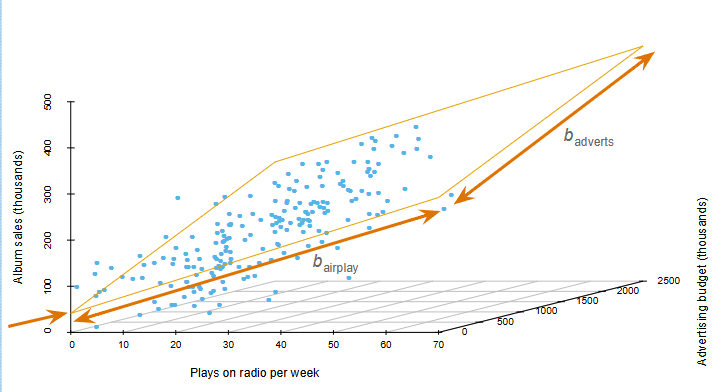
For more predictors needs more dimensions on a graph:
Multicollinearity:
Concept of Multicollinearity:
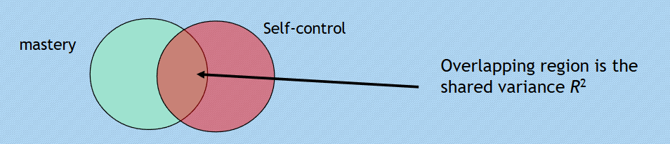
Refers to high correlation between predictors, which can complicate the estimation of the individual predictors.
looks at multiple factors to see which has the most impact of the variable you are interested in
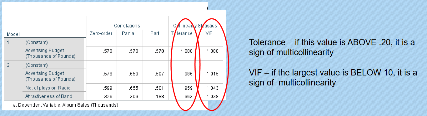
Use Variance Inflation Factor (VIF) and Tolerance for checking multicollinearity:
Tolerance < 0.2 indicates potential multicollinearity issues.
VIF > 10 confirms problematic multicollinearity.

Multiple regression - Assumptions (a priori and post-hoc)
Continuous dv, normal distribution - a priori check (Shapiro wilk test and outlier removal)
Consider bootstrapping / transformation if not normal
Linearity between dependent and independent variables - post-hoc check
Normality of the residual (unexplained variability/ variance in dv) along the IV - post-hoc check
equal variance of the residual along the IV
Hypothesis Testing in Regression
Testing Hypotheses:
Formulating predictions about relationships between variables is essential.
Example Hypothesis: Higher mastery and self-control lead to lower perceived stress.
Hierarchical regression methodologies assess unique contributions of each predictor within this context.
Hierarchical Regression Analysis
Entry Methods
Entry Method: - recommended for assignment
New predictors introduced sequentially to determine each variable's unique predictive power.
Forced Entry:
All variables are entered simultaneously into the model requiring strong theoretical justification for their inclusion.
Model Comparison
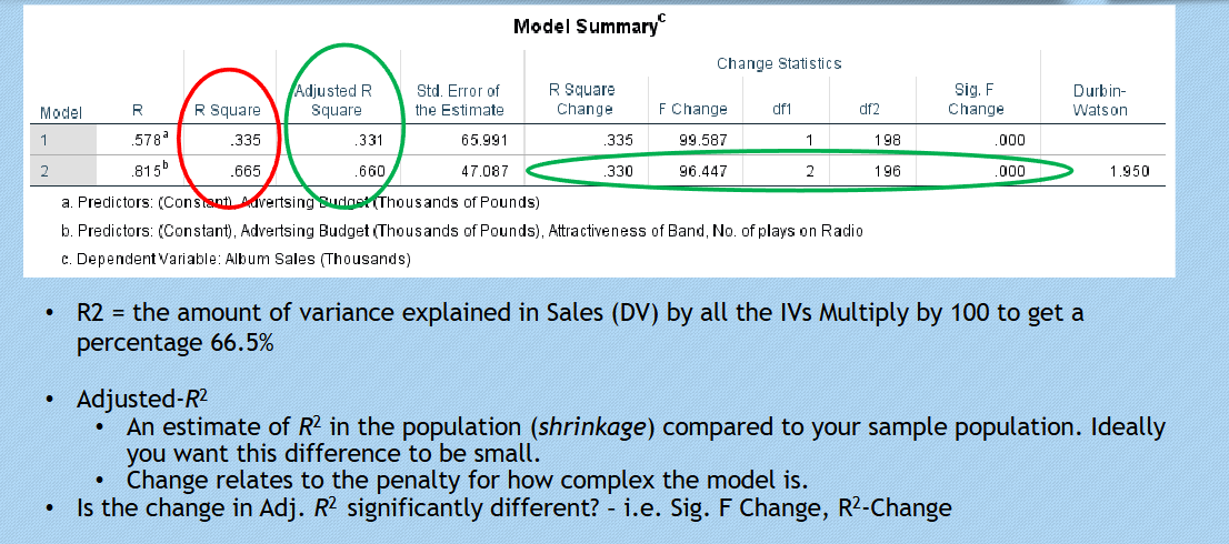
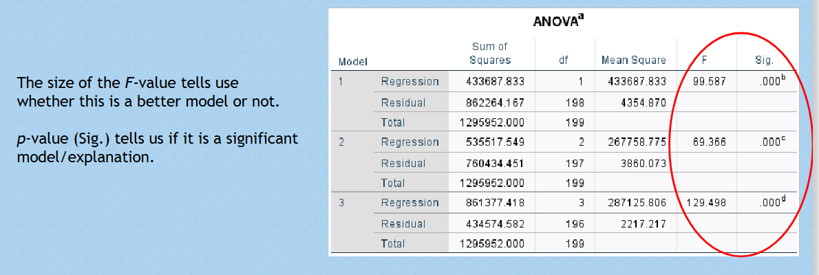
ANOVA F-test:
Used for comparing model fit by determining the amount of variance explained by the model.
F statistics inform about improvements in the model as predictors are added or removed.
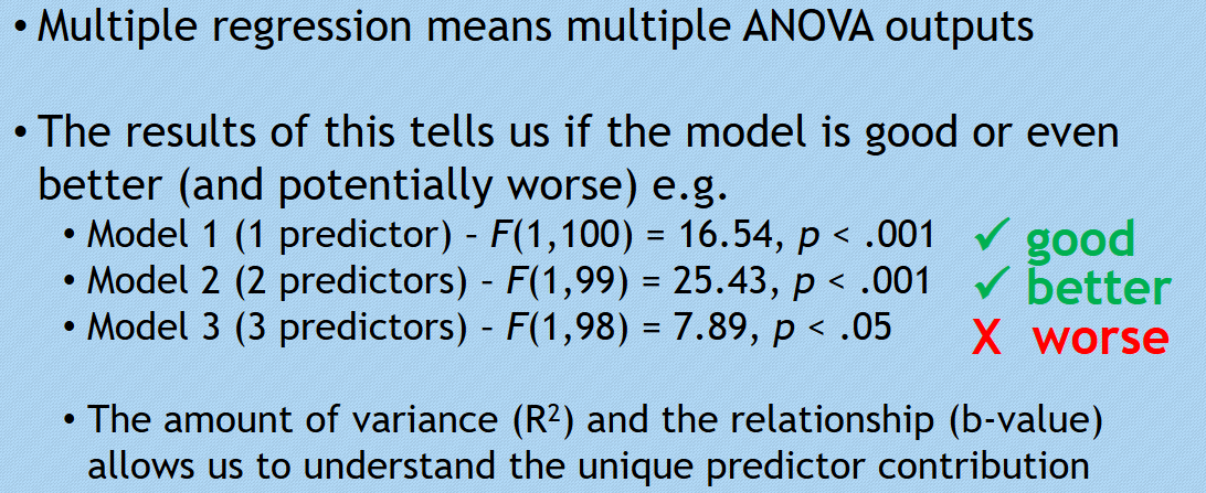
Model 3 shows 3rd predictor added is significant but not as significant as other predictors and so you would not want it in your model.
Practical Application with SPSS
Running Multiple Regression in SPSS
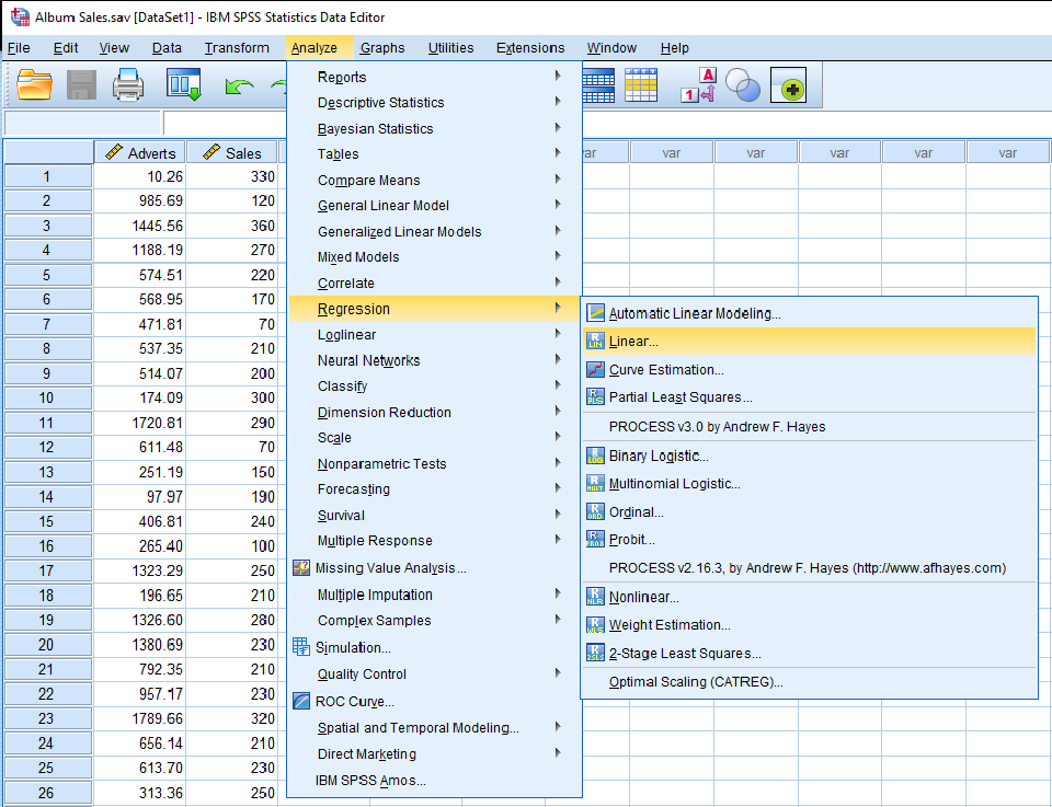
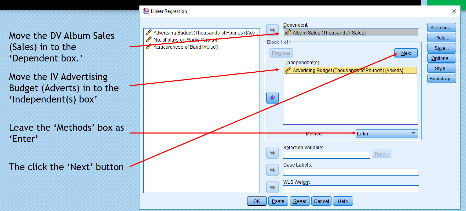
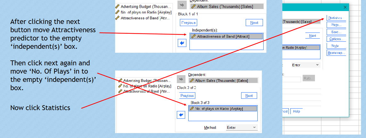
Carefully move DV and IV data into SPSS regression input boxes according to the specifications of the analysis.
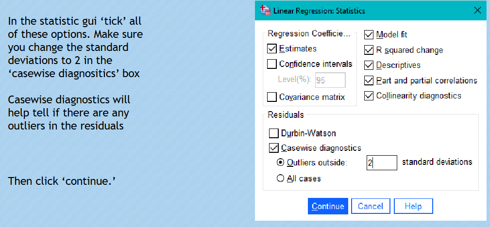
Utilize diagnostics, such as case-wise diagnostics, to analyse and identify outliers that may affect results.
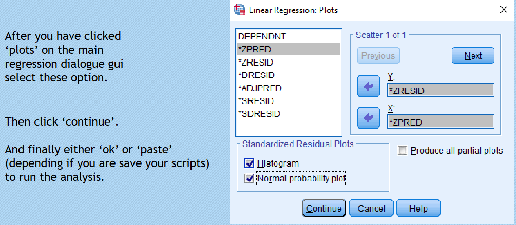
Check assumptions regarding normality of residuals and homoscedasticity through visual tools such as scatterplots.
Interpreting Results
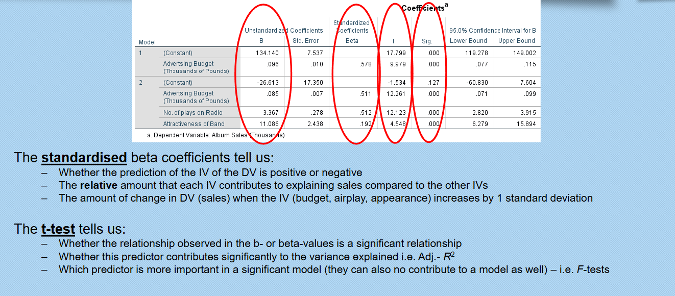
Coefficients indicate relationships and provide insights on contributions of each independent variable to the dependent variable's predictive equation.
Evaluate significance of predictors using t-tests, and assess multicollinearity through tolerance and VIF values.
Reporting Results
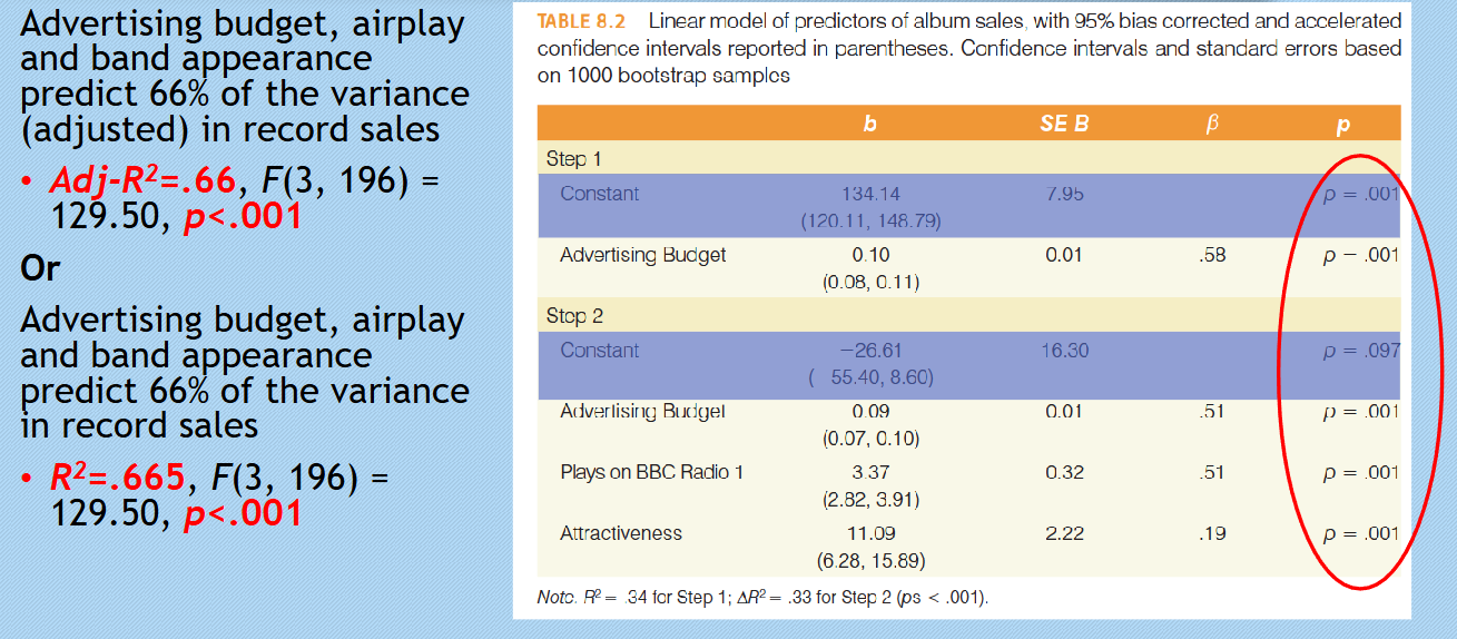
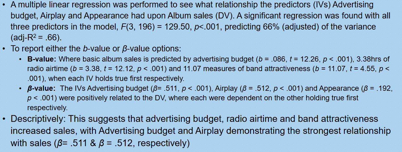
Reporting must include both descriptive statistics and coefficient values to clearly illustrate relationships among variables.
Highlight critical relationships, confirming which factors influence outcomes in the model effectively.
Step by step images bellow:
t-test: Tells us whether the IV is significantly related to the DV (variance explained in this case)
b-values: The relative amount that each IV contributes to explaining sales compared to the other IVs
Standardised b-values : Tell us the same but expressed as standard deviations.
Reporting results
Data quality check
Checks on residuals suggests that there were no violations of normality, with
independence of errors (residuals) confirmed, as the normal plot of the
residuals appeared normality distributed.Homoscedasticity was confirmed via the plot which showed not deviation from
a homoscedastic representation of the residuals. While none of the predictors
showed multicollinearity issues, as VIF and tolerance measures were in range
(< 10 and > 0.2 respectively)