AP Calculus AB Unit 5 Study Guide: Analytical Applications of Differentiation
Interpreting Derivatives in Context (and What They Tell You)
A derivative is more than a rule for computing a slope. The derivative
measures how the output of a function
is changing at the instant when the input is
In other words, it is the instantaneous rate of change of the output with respect to the input. If the function describes a real quantity (height, temperature, profit, position), then its derivative describes how fast that quantity is changing at that moment.
The derivative as slope and as rate
You will use two closely related interpretations throughout this unit.
First, the slope interpretation (geometric):
is the slope of the line tangent to the graph
at
If the tangent line slopes upward to the right then
If it slopes downward then
If it is flat then
Second, the rate interpretation (contextual):
is the instantaneous rate at which
changes with respect to
at
The units are “units of output per unit of input.” For example, if
is position in meters and
is seconds, then
is velocity in meters per second.
A powerful habit is to translate derivative values into sentences with units. If you are told
you should automatically say: “When
the function is increasing at 12 output-units per input-unit.”
Average vs instantaneous rate of change
The average rate of change of
on
is the slope of the secant line:
This is the overall change per input across the whole interval. The derivative is what you get as the interval shrinks to an instant. The Mean Value Theorem later formalizes how average and instantaneous rates are connected.
Using the sign of the derivative to understand behavior
A major theme of Unit 5 is using derivatives to analyze functions without needing an exact graph. If the derivative is positive on an interval, the function is increasing there; if the derivative is negative, the function is decreasing there. If the derivative equals zero at a point, the function has a horizontal tangent there, but that alone does not guarantee a maximum or minimum.
Estimating derivatives from tables and graphs
On the AP exam, you often will not be given a nice formula for
You might get a graph or a table.
From a graph of
estimate
by estimating the slope of the tangent line at
From a table, approximate
using a nearby secant slope, ideally with points equally spaced around
if possible. For example, with data near
one good symmetric estimate is:
The closer the points are to
the better the approximation typically is.
Notation you must recognize
Derivatives appear in several equivalent notations. You need to translate quickly.
| Meaning | Common notations |
|---|---|
| derivative of %%LATEX30%% with respect to %%LATEX31%% | %%LATEX32%%, %%LATEX33%% |
| derivative of | |
| derivative at a point | |
| second derivative | %%LATEX37%%, %%LATEX38%% |
The key idea is that all of these represent rates of change; the notation changes based on context.
Example 1: interpreting a derivative value with units
Suppose
is the temperature of a metal rod (degrees Celsius) at time
minutes. If
then at 5 minutes the temperature is decreasing at 2.3 degrees Celsius per minute. Notice what you should not say: the temperature is not
The derivative is a rate, not the temperature itself.
Example 2: connecting derivative sign to increasing/decreasing
If a graph shows
is below the
-axis for values between 1 and 4, and above the
-axis for values greater than 4, then
is decreasing on
and increasing on
That sign change is a strong hint that
has a local minimum at
(which you justify precisely with the First Derivative Test).
Exam Focus
- Typical question patterns:
- Given a graph or table of %%LATEX51%%, estimate %%LATEX52%% and interpret it in context (including correct units).
- Given a graph of %%LATEX53%%, determine where %%LATEX54%% is increasing/decreasing and identify likely extrema.
- Compare average rate of change on %%LATEX55%% to values of %%LATEX56%%.
- Common mistakes:
- Treating like a function value (confusing “rate” with “amount”). Always include “per unit” language.
- Forgetting units: derivative units are “output units per input unit.”
- Assuming guarantees a maximum or minimum. It only guarantees a horizontal tangent, not the type of extremum.
Critical Points and Local Behavior (Where Extrema Can Happen)
To use derivatives for finding maxima and minima, you need precise vocabulary and a consistent way to identify “places worth checking.”
Local vs absolute extrema
A function can be “highest” or “lowest” in two different ways.
A local maximum at
means that in some open interval around
the value
is greater than or equal to nearby values. A local minimum at
means
is less than or equal to nearby values. These are neighborhood statements, so a local maximum can still be far below an absolute maximum on a larger interval.
An absolute (global) maximum on a domain or interval is the greatest value of
anywhere in that entire set, and an absolute minimum is the least value anywhere in the set.
Critical numbers (where you must look)
Any place an extremum could exist is a critical point, more precisely a critical number (an
-value). A critical number of
is an
-value in the domain of
where either:
or
does not exist.
Critical numbers matter because they are the main interior locations where local extrema can occur (and they are also the interior candidates for absolute extrema when you are restricted to a closed interval).
Why extrema occur at critical numbers (Fermat’s idea)
A key idea (often called Fermat’s Theorem) is: if
has a local maximum or local minimum at
and
exists, then:
Intuitively, if you are at the top of a smooth hill, the tangent line must be flat.
Two important caveats drive many AP mistakes. First, the converse is false: a point where
might be a “flat spot” with no extremum. Second, derivatives can fail to exist at extrema: corners and cusps can still produce local maxima or minima.
Endpoints are not “critical numbers” but still matter
On a closed interval
endpoints
and
can produce absolute extrema even though the usual two-sided neighborhood idea for “local” extrema does not apply at an endpoint. You treat endpoints separately when searching for absolute extrema.
Example 1: finding critical numbers from a formula
Let
Then
Set the derivative equal to zero:
Both
and
are critical numbers.
Example 2: a critical number where the derivative does not exist
If
then
has a sharp corner at
The derivative does not exist at 0, but 0 is still a critical number, and it is also a local minimum.
Exam Focus
- Typical question patterns:
- Identify critical numbers of from a graph (horizontal tangents, corners, cusps) or from a derivative.
- Decide whether given points could contain local extrema based on whether %%LATEX91%% or %%LATEX92%% is undefined.
- Distinguish local vs absolute extrema in words or from a graph.
- Common mistakes:
- Looking only for %%LATEX93%% and forgetting points where %%LATEX94%% does not exist.
- Treating endpoints as critical numbers and applying local-extrema logic incorrectly. Endpoints are checked for absolute extrema on closed intervals, but they are not “local extrema” in the same two-sided sense.
- Assuming every critical number is an extremum. You must test behavior around the critical number.
Absolute Extrema on Closed Intervals: Extreme Value Theorem and the Candidates Test
When you are asked for the absolute maximum or minimum on an interval, you need (1) a guarantee that such values exist and (2) a reliable method to find them.
Extreme Value Theorem (EVT): what it says and why it matters
The Extreme Value Theorem states that if a function is continuous on a closed interval, then it must have both a maximum and a minimum value on that interval. These maximum and minimum values are called extrema.
Formally:
If
is continuous on
then
attains both an absolute maximum value and an absolute minimum value on
This is an existence theorem: it does not tell you where the extrema occur.
Why the conditions matter: the interval must be closed (endpoints included) and the function must be continuous on that interval (no holes, jumps, or asymptotes inside). If either condition fails, an absolute max or min might not exist. For example, on the open interval
the function
has no absolute minimum or maximum because it never reaches 0 or 1.
The Closed Interval Method (Candidates Test)
To actually find absolute extrema on
you use the Closed Interval Method, also called the Candidates Test.
- Confirm you are working on a closed interval
- Find all critical numbers of
in
- Make a table of the endpoints and the critical numbers.
- Plug each candidate back into the original function
(not the derivative) to get the corresponding function values.
- Compare the values: the largest is the absolute maximum value and the smallest is the absolute minimum value.
The method works because on a closed interval, absolute extrema must occur either at interior points where the derivative is zero/undefined or at endpoints.
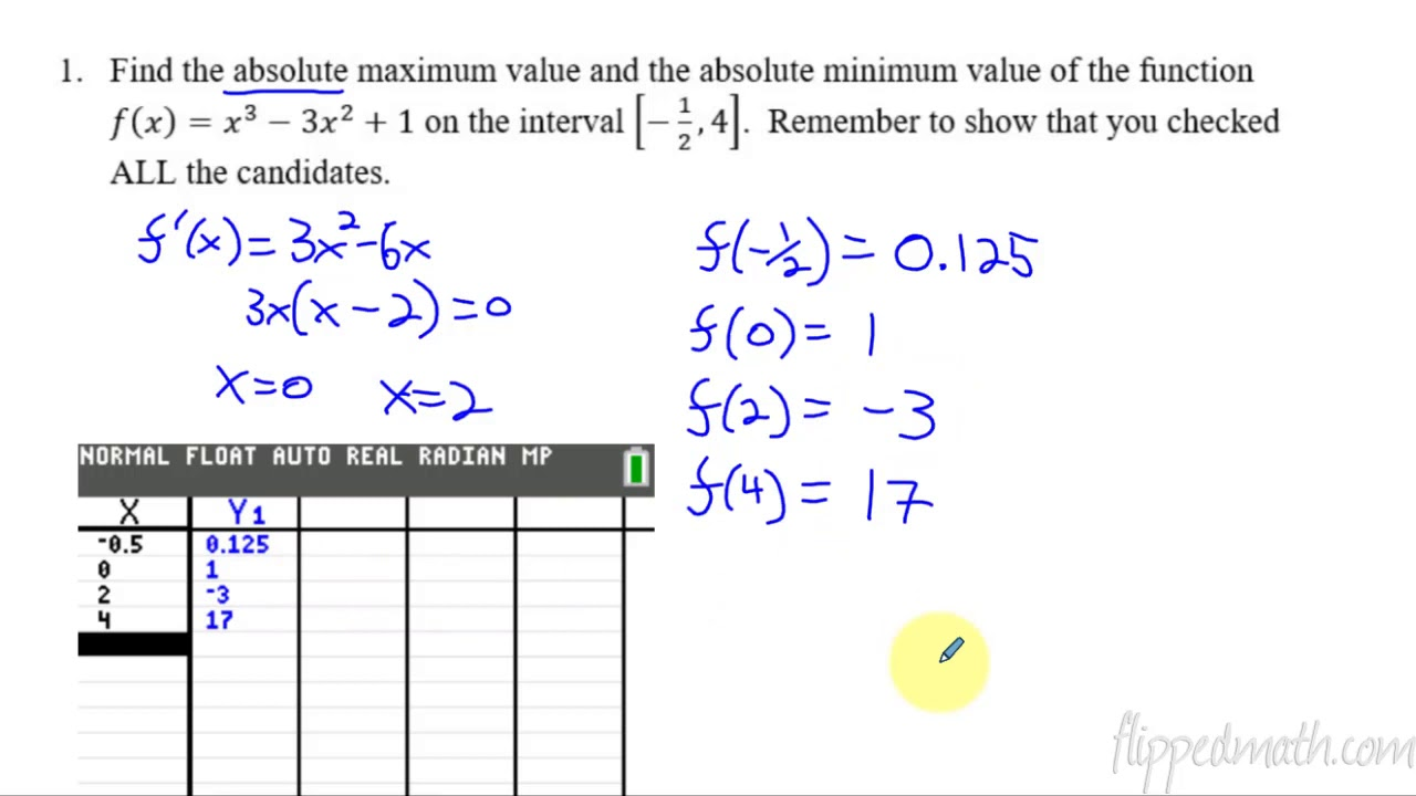
Example: absolute max/min using the candidates test
Find the absolute extrema of
on
Critical numbers come from
so
and
Now evaluate the original function at endpoints and critical numbers:
The maximum value is
(occurs at
and
). The minimum value is
(occurs at
and
). This also highlights an AP point: absolute extrema can occur at multiple
-values.
When you must not use EVT/candidates test blindly
If the function is not continuous on
then EVT does not apply and absolute extrema might not exist. If the interval is not closed (for example
), the Closed Interval Method is not a guarantee. On AP questions, they often explicitly state continuity on
when they want you to cite EVT.
Exam Focus
- Typical question patterns:
- “Show that %%LATEX125%% has an absolute maximum and minimum on %%LATEX126%%.” (Use EVT: continuity plus closed interval.)
- “Find the absolute maximum value of %%LATEX127%% on %%LATEX128%%.” (Use candidates test: endpoints plus critical numbers.)
- Tables/graphs: compare function values at listed candidates.
- Common mistakes:
- Forgetting to check endpoints when asked for absolute extrema on .
- Listing critical numbers but not evaluating %%LATEX130%% at them (the extremum is a function value, not just an %%LATEX131%%-value).
- Using EVT when continuity or the closed-interval condition is missing.
Mean Value Theorem and Rolle’s Theorem (Bridging Average and Instantaneous Change)
The Mean Value Theorem (MVT) is one of the most important “big picture” results in differential calculus because it links the average rate of change on an interval to the instantaneous rate of change at a point. In other words, there must be some point in the interval where the slope of the tangent line equals the slope of the secant line that connects the endpoints.
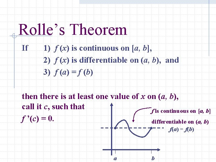
Rolle’s Theorem: the special case
Rolle’s Theorem is a special case of the MVT. It says: if
is continuous on
, differentiable on
, and
, then there exists at least one number
in
such that:
Interpretation: a continuous, differentiable curve must have a horizontal tangent between two points where it starts and ends at the same height.
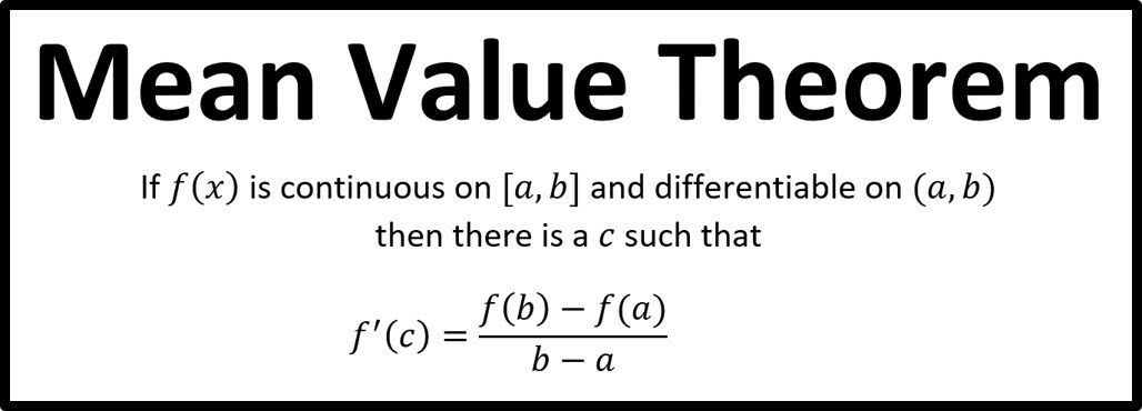
Mean Value Theorem: the general version
The Mean Value Theorem says: if
is continuous on
and differentiable on
, then there exists at least one number
in
such that:
The right-hand side is the average rate of change, so MVT guarantees that somewhere in the interval, the instantaneous rate equals the average rate.
Why this matters: it justifies “there exists a point where…” reasoning, it supports the idea that if the derivative is zero everywhere then the function is constant, and it is central to many AP free-response justifications.
Understanding the hypotheses (what you must check)
MVT requires both continuity on the closed interval and differentiability on the open interval. Corners, cusps, vertical tangents, or discontinuities inside
break the hypotheses, and then the conclusion is not guaranteed.
Example 1: finding the point(s) guaranteed by MVT
Let
on
Compute the average rate of change:
Compute the derivative:
Set the derivative equal to the average slope:
So MVT guarantees at least one point, and here it is.
Example 2: recognizing when MVT does not apply
Consider
on
The function is continuous on the closed interval but not differentiable at
inside the interval, so MVT does not apply. You cannot claim there must be a point
where:
Exam Focus
- Typical question patterns:
- “Verify that MVT applies on %%LATEX157%% and find all values of %%LATEX158%% that satisfy the conclusion.”
- “Explain why there exists a point %%LATEX159%% where %%LATEX160%%.” (Often compute an average slope and cite MVT.)
- “Does MVT apply?” based on continuity/differentiability from a graph.
- Common mistakes:
- Checking continuity but forgetting differentiability on the open interval.
- Using Rolle’s Theorem when %%LATEX161%% and %%LATEX162%% are not equal.
- Solving for %%LATEX163%% but giving a value outside %%LATEX164%%.
Increasing/Decreasing and the First Derivative Test (How Sign Charts Create Conclusions)
Once you know where a derivative is positive or negative, you can turn that into a complete “story” of the function. This includes intervals of increase and decrease and the classification of relative (local) extrema.
Monotonicity: formal meaning of increasing/decreasing
Using the first derivative, you can identify when the original function is increasing or decreasing. Where the derivative is positive, the function is increasing; where the derivative is negative, the function is decreasing. This is one of the most-used tools in Unit 5 because it translates calculus into graph shape.
Building a sign chart from the first derivative
A sign chart is a structured way to track where the derivative is positive, negative, or zero.
A standard AP-friendly procedure is:
- Take the derivative of the function.
- Set it equal to zero to find critical numbers (and also note where the derivative is undefined).
- Plug in a test value above each critical number and below it (more generally, one test point in each interval) to determine the sign of the derivative.
The image below illustrates the “test a point on each side” idea:
The First Derivative Test (for relative extrema)
The first derivative also tells you relative (local) maxima and minima.
Let
be a critical number.
- If the derivative shifts from positive to negative at
then the function changes from increasing to decreasing, so there is a relative (local) maximum at
- If the derivative shifts from negative to positive at
then the function changes from decreasing to increasing, so there is a relative (local) minimum at
- If there is no sign change, there is no local extremum at that critical number.
Example 1: using the first derivative test (sign-chart approach)
Let
Then
Critical numbers:
and
Testing intervals:
- On
pick
and get a positive derivative, so the function is increasing.
- On
pick
and get a negative derivative, so the function is decreasing.
- On
pick
and get a positive derivative, so the function is increasing.
Therefore, the derivative changes from positive to negative at
(local maximum) and from negative to positive at
(local minimum).
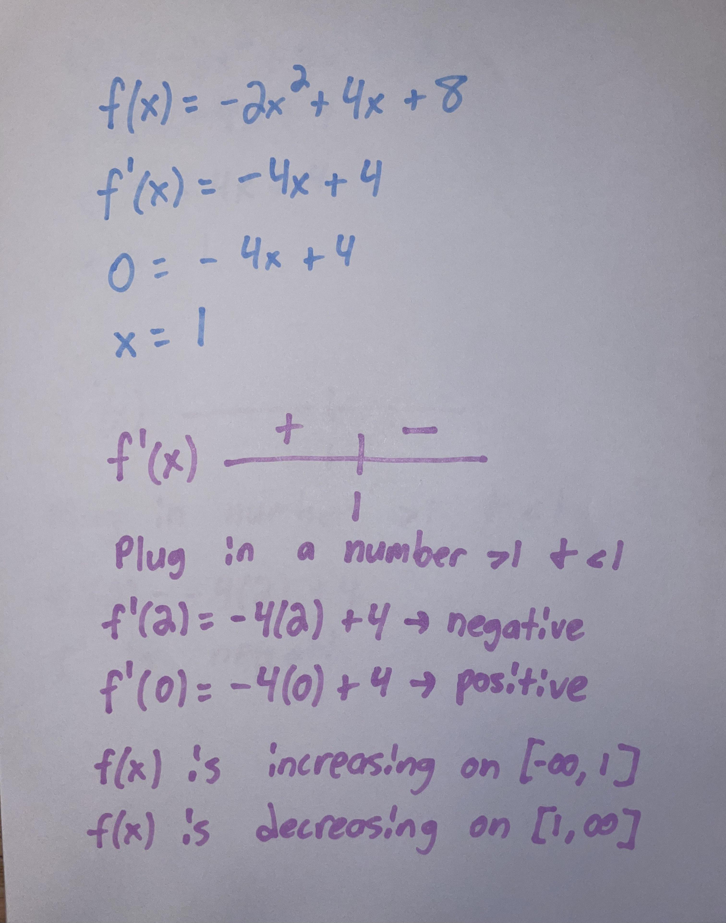
Example 2: intervals of increase/decrease for a polynomial (from a common AP pattern)
Let
Differentiate:
Set the derivative equal to zero:
Factoring gives critical numbers:
and
Now test the sign of the derivative in each interval.
- For
pick
Then
so the function is increasing on
- For
pick
Then
so the function is decreasing on
- For
pick
Then
so the function is increasing on
So the function increases, then decreases, then increases. That means there is a relative (local) maximum at
(positive to negative) and a relative (local) minimum at
(negative to positive).
A frequent subtlety: critical points with no extremum
A classic example is
Then
and
but the derivative is nonnegative on both sides of 0 and does not change sign, so there is no local max or min at 0.
Exam Focus
- Typical question patterns:
- Given %%LATEX204%% (formula, graph, or table), find intervals where %%LATEX205%% is increasing/decreasing.
- Use a sign chart to identify local maxima/minima and justify with the First Derivative Test.
- Interpret monotonicity in context (for example, “profit increases for ”).
- Common mistakes:
- Declaring “max” or “min” from without checking sign change.
- Forgetting that if %%LATEX208%% is undefined at %%LATEX209%% but %%LATEX210%% is defined, %%LATEX211%% is still a critical number.
- Mixing up the sign-change directions: positive to negative is a maximum; negative to positive is a minimum.
Concavity, Inflection Points, and the Second Derivative (How the Slope Itself Changes)
The first derivative tells you whether a function is increasing or decreasing. The second derivative tells you whether that increase or decrease is happening at an increasing rate or a decreasing rate. A function can be increasing but “slowing down,” and concavity is the language that describes this.
What concavity means in plain language
A function is concave up when its graph bends like a cup; tangent lines tend to lie below the graph. A function is concave down when it bends like a cap; tangent lines tend to lie above the graph.
A useful slope-based interpretation is: concave up means slopes are increasing as you move right, and concave down means slopes are decreasing as you move right.
The second derivative and what it measures
The second derivative
is the derivative of
so it measures the rate of change of the slope.
- If
on an interval, the function is concave up there.
- If
on an interval, the function is concave down there.
In context, if
is position, then
is velocity and
is acceleration. Positive acceleration corresponds to velocity increasing, which lines up with concave up behavior.
A common visual summary:
Inflection points (where concavity changes)
An inflection point is a point on the graph where concavity changes (from concave up to concave down or vice versa).
Candidates for inflection points occur where:
or where
does not exist. However, you only confirm an inflection point if the concavity actually changes sign across that value.
A standard procedure (mirroring first-derivative sign charts) is:
- Take the second derivative.
- Set it equal to zero to find possible inflection points.
- Check the sign of the second derivative on each side to verify whether it changes sign.
Second Derivative Test (classifying critical points)
The Second Derivative Test is a shortcut for classifying a critical number
where
- If
then the graph is concave up there, so the point is a local minimum.
- If
then the graph is concave down there, so the point is a local maximum.
- If
(or does not exist), the test is inconclusive.
Example 1: concavity and an inflection point
Let
Then
and
For
,
so the function is concave down. For
,
so it is concave up. At
,
and concavity changes sign, so there is an inflection point at
This also shows a key idea: a point can be a critical number (since
) but not a max or min, and still be an important shape feature.
Example 2: second derivative test in action
Let
Then
Critical numbers:
,
,
Now
Evaluate:
so there is a local maximum at
Also,
so there is a local minimum at
And
so there is a local minimum at
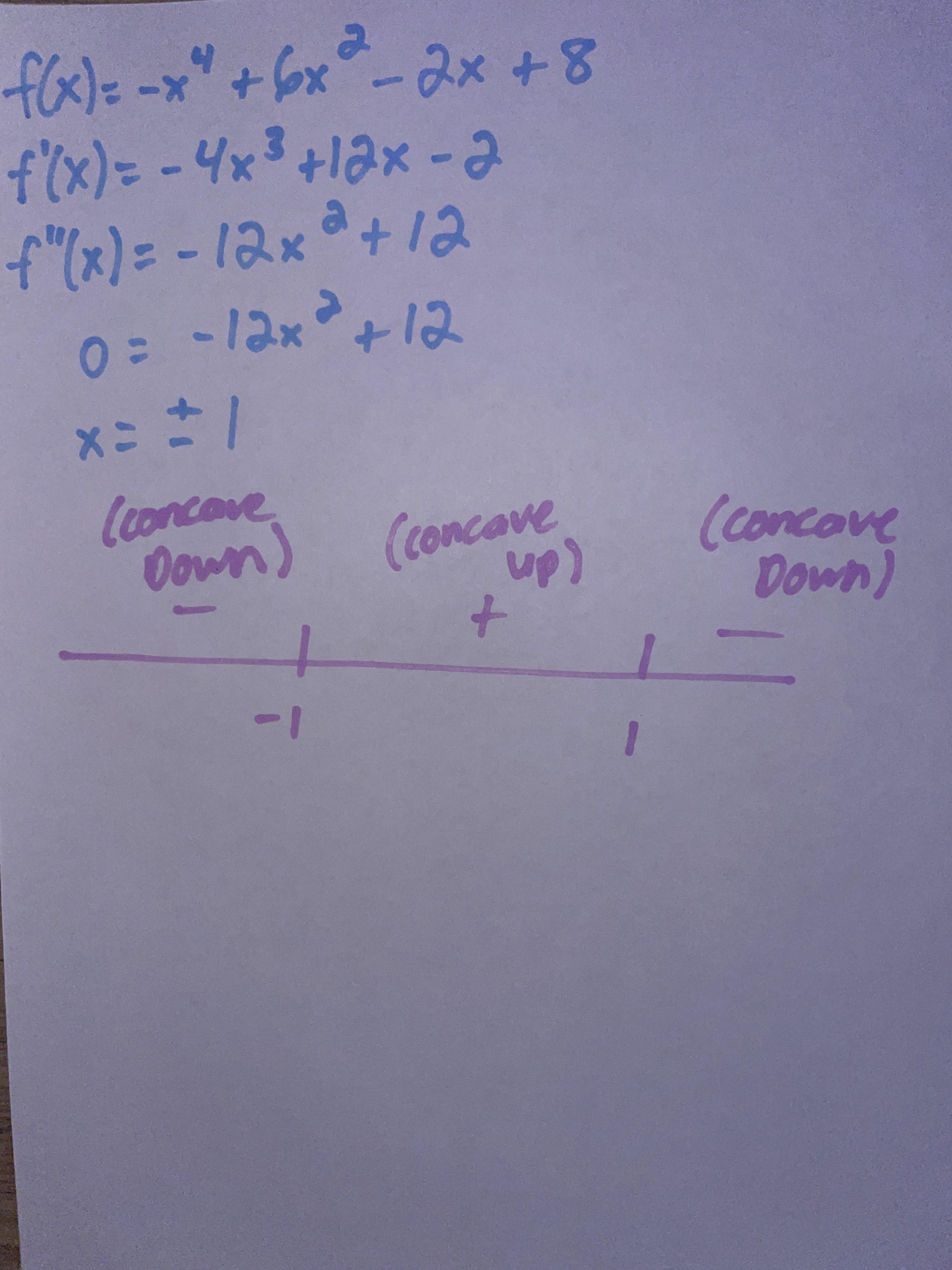
Example 3: concavity intervals for a polynomial
Using the earlier polynomial
we already found
Now take the second derivative:
Set it equal to zero to find the possible inflection point:
Test the sign:
- If
then
so the function is concave down on
- If
then
so the function is concave up on
Because the concavity changes at
, the graph has an inflection point there.
Exam Focus
- Typical question patterns:
- Given %%LATEX261%% (or a graph of %%LATEX262%%), find where is concave up/down and where inflection points occur.
- Use the Second Derivative Test to classify critical points when appropriate.
- Interpret concavity in context (for example, “the rate of increase is accelerating”).
- Common mistakes:
- Declaring an inflection point just because without checking a concavity change.
- Confusing increasing/decreasing with concavity: increasing is about the sign of %%LATEX265%%; concavity is about the sign of %%LATEX266%%.
- Using the Second Derivative Test when . The test is specifically about critical points with horizontal tangents.
Optimization (Max/Min Modeling with Calculus)
Optimization problems ask you to choose the “best” option under constraints: maximize profit, minimize cost, minimize material, maximize area, and so on. In calculus, “best” typically means an absolute maximum or absolute minimum of an objective function on an appropriate domain.
The big idea behind calculus optimization
Optimization is not about memorizing a different formula for every scenario; it is about modeling.
- Identify the quantity you want to optimize (the objective function).
- Use the constraints to rewrite the objective as a single-variable function.
- Determine the feasible domain (often a closed interval from physical constraints).
- Find critical numbers and test candidates (often with the Closed Interval Method).
Derivatives show up because interior maxima and minima occur at critical numbers, where the derivative is zero or undefined.
Step-by-step optimization strategy (what to do and why)
Step 1: Draw a picture and define variables. A diagram prevents algebra mistakes.
Step 2: Write the objective function. At first it may involve multiple variables.
Step 3: Use constraints to reduce to one variable. Substitute until you have a single-variable function.
Step 4: Identify the feasible domain. Lengths must be positive, and constraints often create an upper bound too.
Step 5: Differentiate and find critical numbers. Solve
and check where the derivative is undefined.
Step 6: Justify max/min. On a closed interval, use the candidates test. On an open interval, justify with first/second derivative tests and context.
Step 7: Answer in context. State the optimized dimensions and the optimized value with units.
A frequent AP scoring issue is doing the calculus correctly but not answering what was asked (for example, giving only the
-value but not the maximum area).
Example 1: maximizing area with fixed perimeter
You have 100 meters of fencing to make a rectangle. What dimensions maximize the area?
Let width be
and length be
Constraint:
so
Objective (area):
Substitute:
Domain:
Differentiate:
Set to zero:
Candidates test at
,
,
:
So the maximum occurs at
and
The maximum-area rectangle is a square. Symmetry often appears in optimization, but you still justify it with calculus.
Example 2: minimizing material (open-top box)
Build a box with a square base and no top, volume 32 cubic units. Minimize material used.
Let base side length be
and height be
Constraint:
so
Objective (surface area without top):
Substitute:
Domain:
Differentiate:
Set equal to zero:
Then
To justify it is a minimum, you can argue end behavior
as
and as
so the interior critical point must be the global minimum, or you can use the second derivative:
Since
the function is concave up there, confirming a minimum.
Common modeling pitfalls in optimization
Mixing up what is fixed and what varies is a common error (for example, treating perimeter as variable when it is constant). Other frequent issues are forgetting to reduce to one variable before differentiating, using dimensions outside the feasible domain (like negative lengths), and concluding “minimum” just because you found a critical point without justification.
Exam Focus
- Typical question patterns:
- Geometry optimization: maximize area, minimize surface area, minimize distance.
- Applied optimization: maximize revenue/profit with a given demand model; minimize cost.
- Justification prompts: “Show that the function has a minimum on the given interval” (often EVT) and “find the minimum value.”
- Common mistakes:
- Providing the optimizing -value but not the maximum/minimum value of the objective.
- Forgetting endpoints when the feasible domain is a closed interval.
- Algebra errors in constraint substitution (a small mistake early can ruin the derivative step).
Putting It All Together: Analyzing a Function’s Graph Using Derivatives
Many Unit 5 problems are synthesis problems: you are given a function (or derivative information) and asked to describe behavior (increase/decrease, concavity, extrema, inflection points) and sometimes sketch a graph consistent with that information. The goal is not artistic graphing; it is building a logically consistent shape supported by derivative evidence.
A structured analysis workflow
A consistent workflow helps you avoid missing features:
- Domain and important points: where is the function defined, and are there endpoints that must be checked?
- First derivative features:
- critical numbers where
or
is undefined
- intervals where the derivative is positive or negative
- local maxima/minima using the First Derivative Test
- Second derivative features:
- possible inflection points where
or
is undefined
- intervals where the second derivative is positive or negative
- confirm inflection points by checking for a sign change
A key connection: concavity is about whether the first derivative is increasing or decreasing.
- If the function is concave up, then
is increasing.
- If the function is concave down, then
is decreasing.
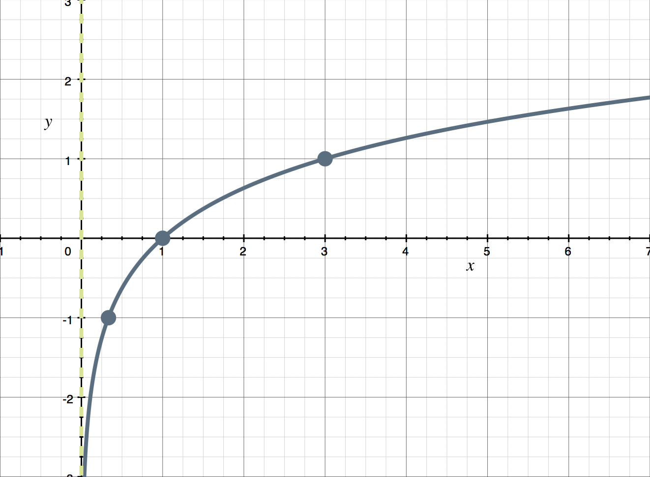
Reading the original function from a graph of the derivative
If you are given a graph of
instead of
:
- Where
, the function is increasing.
- Where
, the function is decreasing.
- Where
and changes sign, the function has a local extremum.
- Where the graph of
is increasing, the function is concave up.
- Where the graph of
is decreasing, the function is concave down.
This last pair is powerful: you can determine concavity from the shape of
without explicitly computing
Example: full analysis from a function
Analyze
First derivative:
Critical numbers:
and
The derivative is positive for
, negative for
, and positive for
So there is a local maximum at
and a local minimum at
Second derivative:
Concavity: concave down for
and concave up for
Because concavity changes at
, there is an inflection point at
Example: determining shape from a graph of the derivative (conceptual)
Suppose the graph of
crosses the
-axis at
and
and suppose:
on
,
on
, and
on
Then the function increases, then decreases, then increases, so there is a local maximum at
and a local minimum at
Now suppose the graph of
is increasing on
and decreasing on
Then the function is concave up on
and concave down on
So
is an inflection point of the original function (because concavity changes there).
What “justify your answer” usually means here
On AP free-response, you are expected to explicitly connect claims to derivative-based reasons. Examples of acceptable justification sentences include:
- “The function is increasing on an interval because the derivative is positive on that interval.”
- “The function has a local maximum at
because the derivative changes from positive to negative at
.”
- “The function is concave down on an interval because the second derivative is negative on that interval.”
The vocabulary is part of the grade: state the sign information and state what it implies.
Exam Focus
- Typical question patterns:
- Given , find intervals of increase/decrease, concavity, local extrema, and inflection points.
- Given a graph of %%LATEX358%% (or %%LATEX359%%), infer features of and justify each claim.
- Free-response “analysis” questions that require written reasoning with derivative tests.
- Common mistakes:
- Confusing the graph of %%LATEX361%% with the graph of %%LATEX362%% (for example, thinking %%LATEX363%% is the %%LATEX364%%-value of ).
- Declaring extrema at every place where without checking sign changes.
- Declaring inflection points at every place where without checking concavity change.