B4.2 Ecological Niches
Chapter 1: Interactions with the environment
Key Information for Exam:
Specialist vs. Generalist Species:
Specialist species: Survive in narrow, specific environments (e.g., Koala only feeds on eucalyptus leaves).
Generalist species: Can survive in a broader range of environments (e.g., Black rats).
Ecological Niche:
Refers to where an organism lives, what it does, and its role in the ecosystem. It’s influenced by biotic factors (e.g., competition, disease, predators) and abiotic factors (e.g., temperature, water, soil).
Example: Bryophytes need moderate temperatures, water, and indirect light, while cactus needs less water and can grow in poor soil.
Impact of Species on Environment:
Beavers: Create wetlands by building dams, which increase biodiversity.
Worms: Improve soil quality by breaking down organic matter, enhancing nutrient content, and drainage.
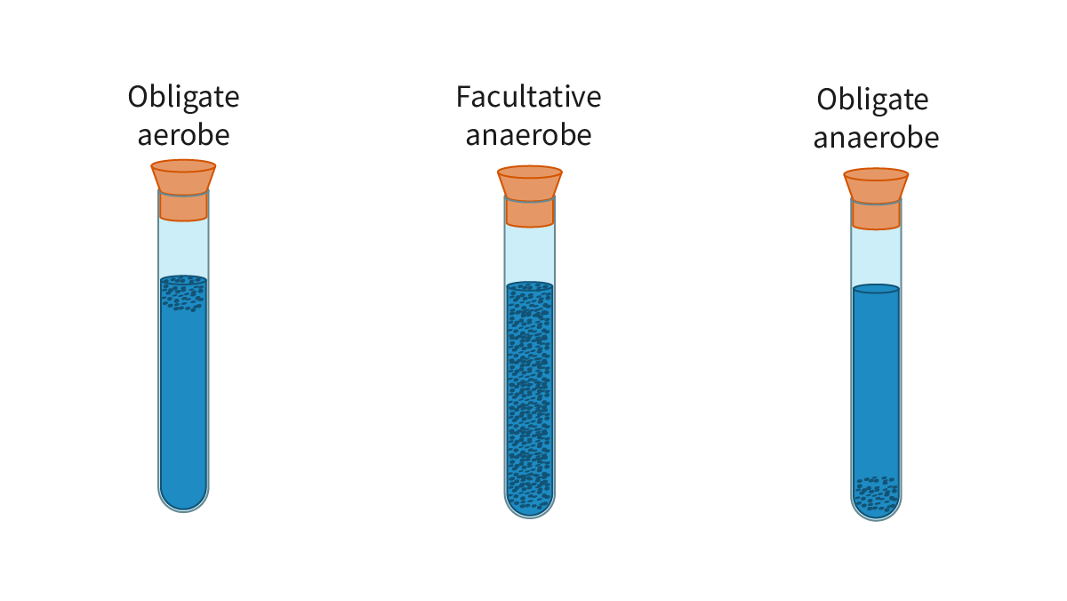
Modes of Respiration:
Obligate Anaerobes: Do not survive in oxygen; use compounds like sulfate or nitrates (e.g., Clostridium difficile).
Facultative Anaerobes: Can use both oxygen and fermentation for energy (e.g., Escherichia coli).
Obligate Aerobes: Require oxygen for respiration (e.g., Mycobacterium tuberculosis).
Experiment for Respiration Types: Bacteria grow in culture medium with varying oxygen levels. Anaerobes move to the bottom, aerobes to the top, and facultative anaerobes in between.
Chapter 2: Nutrition
Nutrition Types:
Producers (Autotrophs): Organisms that generate their own nutrition (e.g., plants, algae, some prokaryotes).
Consumers (Heterotrophs): Organisms that take in nutrition from external sources (e.g., animals, humans).
Photosynthetic Nutrition:
Autotrophs use sunlight to generate energy via photosynthesis.
Photosynthesis equation:
6CO2+6H2O→C6H12O6+6O2\text{6CO}_2 + \text{6H}_2\text{O} \rightarrow \text{C}_6\text{H}_{12}\text{O}_6 + \text{6O}_26CO2+6H2O→C6H12O6+6O2Chloroplasts (found in plant leaves, algae, etc.) are responsible for capturing light energy.
Holozoic Nutrition:
Heterotrophic organisms that take in solid/liquid food (e.g., most animals, protozoa).
Food is ingested, digested, and used for growth and development.
Mixotrophic Nutrition:
Organisms that combine autotrophic and heterotrophic methods (e.g., marine plankton).
Facultative mixotrophs can switch between the two methods; obligate mixotrophs must use both.
Saprotrophic Nutrition:
Organisms (e.g., fungi, bacteria) break down dead organic material using digestive enzymes.
Important for recycling nutrients in ecosystems.
Nutrition in Archaea:
Archaea are unicellular organisms that differ from bacteria in biochemistry and cell walls.
Some are chemoautotrophs, using inorganic chemicals for energy; others are photoautotrophs or heterotrophs.
Many archaea are extremophiles (live in extreme environments like hot springs, deep sea vents).
Chapter 3: Dentition
Cookiecutter Shark (Isistius brasiliensis):
Known for creating circular "cookie-cutter" wounds in prey using specialized teeth.
Small shark with adult males reaching 42 cm.
Teeth: 30–37 small upper teeth and 25–31 larger triangular lower teeth.
Shark attaches to prey, generates a vacuum, and uses a rotation to remove a circular chunk of flesh.
Teeth and Diet Studies:
Dental Microwear: Marks on teeth can indicate an organism's diet.
Isotope Analysis: Used to study the diet of extinct mammals through skeletal elements like carbon, calcium, and strontium.
Hominids and Hominins:
Hominids: Include all great apes and humans (e.g., gorillas, orangutans, chimpanzees).
Hominins: Refers to modern humans and their immediate ancestors.
Humans are generalists with diverse diets, capable of consuming both plants and animals.
Early hominin dentition shows a trend from larger teeth (for chewing fibrous plants) to smaller teeth as meat consumption increased.
Early Hominin Groups:
Archaic Megadont Hominins (e.g., Paranthropus robustus):
Lived 1.8 to 1.2 million years ago.
Large teeth, thick enamel, strong jaw muscles, and wide faces.
Believed to have been herbivores, consuming tough grasses and fibrous plants.
Pre-modern Homo (e.g., Homo floresiensis and Homo sapiens):
Homo floresiensis ("Hobbit"):
Lived between 100,000 and 50,000 years ago.
Small in size, with large teeth for their skull size.
Likely omnivores, with evidence of a fibrous diet requiring much chewing.
Homo sapiens:
Evolved around 300,000 years ago.
Smaller jaws and teeth, adaptable to varied diets and environments.
Key Hominin Evolution Trends:
Over time, faces became more vertical, canines and jaws became shorter.
Modern humans (Homo sapiens) have tightly arranged teeth in a U-shape.
Exam Focus:
Cookiecutter shark feeding behavior and dentition.
Evolution of hominin dentition linked to diet and energy needs.
Key differences between early hominins (e.g., Paranthropus robustus) and modern humans (Homo sapiens).
Chapter 4: Adaptations
Herbivores:
Herbivores are animals that eat only plants, including invertebrates, cows, goats, buffalo, and even hippos.
Hippos are the most dangerous land mammals, killing more people than lions and other large predators.
Herbivore Adaptations:
Insects: Use specialized mandibles or stylets (e.g., aphids) to feed on plant fluids.
Mammals: Herbivorous mammals, like cows or goats, have long, flat front incisors to cut plants, and large flat molars for grinding. The diastema (gap between incisors and molars) allows for effective food movement.
Teeth Growth: Herbivores, like hippos, have continuously growing teeth. Hippos' canine and incisor teeth can grow up to 50 cm in length and are used for defense or combat, not feeding.
Wide-set Eyes: Many herbivores have eyes placed far apart to increase their visual field, helping them detect predators early.
Plant Defenses Against Herbivores:
Toxic Secondary Compounds: Some plants produce chemicals that are toxic to herbivores (e.g., terpenes, phenolics, alkaloids). Examples include artemisinin (anti-malaria) and paclitaxel (anti-cancer).
Animal-Plant Warfare: Plants evolve chemical defenses, while herbivores may evolve enzymes to metabolize these toxins.
Structural Defenses: Plants may have thick leaves, spiny thorns, or microscopic thorns (e.g., trichomes) to deter herbivores.
Mimicry: Some plants, like Lithops (living stones), avoid predation by blending into their surroundings.
Predator Adaptations:
Physical: Predators use speed, claws, sharp teeth, and fine-tuned senses (e.g., an eagle can spot prey from 3 km away) to hunt.
Chemical: Some predators, like Brazilian fire ants or cone snails, use venom to immobilize or kill their prey.
Behavioral: Dolphins, for example, work together to trap fish with a mud ring, while Margay cats mimic distress calls to lure prey.
Prey Adaptations to Avoid Predation:
Physical: Camouflage (e.g., zebra stripes), speed and agility, and defense mechanisms like spines (e.g., hedgehogs).
Chemical: Prey like skunks release noxious smells to deter predators, while some prey release toxic chemicals to harm predators.
Behavioral: Species like mackerel form balls to confuse predators and reduce individual risk.
Plants' Adaptations to Harvest Light:
Lianas: Climbing plants that can reach the canopy by growing along tall trees.
Epiphytes: Plants like the strangler fig grow on other plants, obtaining water from the host plant rather than the soil.
Shade Tolerance: Plants in forest ecosystems, like those in the herb layer, have adaptations (e.g., large thin leaves) to maximize light absorption in low-light environments.
Exam Focus:
Herbivore feeding strategies and physical adaptations (e.g., teeth structure and growth).
Plant defenses against herbivores and how herbivores adapt to these defenses.
Predator adaptations in hunting, including chemical and behavioral methods.
Prey adaptations to avoid being eaten, such as physical defense mechanisms and group behaviors.
Plant adaptations to obtain light in forest ecosystems, including epiphytic and liana plants.
Chapter 5: Competitive Exclusion
Fundamental and Realised Niches:
Fundamental Niche: The ideal environmental conditions where an organism can live and reproduce, considering both abiotic (non-living) and biotic (living) factors.
Realised Niche: The actual living and reproducing conditions of an organism, which are constrained by factors like competition with other species. The realised niche is smaller than the fundamental niche due to these pressures.
Example: Coyotes and wolves in North America. The fundamental niche for coyotes was large, but due to competition from wolves, the realised niche for coyotes was smaller. When wolves were hunted by settlers, coyotes’ realised niche expanded.
Competitive Exclusion Principle (Gause’s Law):
Competitive Exclusion: Two species cannot occupy the same niche indefinitely. One species will outcompete the other. Over time, competition for resources results in the exclusion or adaptation of one species.
Example: Paramecium aurelia and Paramecium caudatum are protozoans that compete for the same resources. When grown together, P. aurelia outcompetes P. caudatum, leading to the latter's extinction.
Niche Partitioning:
Niche partitioning refers to the way competing species adapt to share a habitat by occupying different niches or parts of the same niche.
Spatial Partitioning: Species evolve to use different physical spaces within the same habitat, reducing competition for resources.
Example: Warbler birds (MacArthur, 1956) occupy different heights on coniferous trees, each with distinct food requirements and nesting times.
Temporal Partitioning: Species evolve to use the same area at different times, reducing direct competition for resources.
Example: In the deserts of Israel, the common spiny mouse is nocturnal, and the golden spiny mouse is diurnal. This temporal partitioning allows both species to coexist in the same habitat.
Exam Focus:
Understand the differences between fundamental and realised niches and how the realised niche is influenced by competition and environmental pressures.
Know the competitive exclusion principle and how it explains why species cannot coexist in the same niche over time.
Familiarize with niche partitioning, both spatial and temporal, as strategies that allow species to coexist in similar environments.
1. The Chi-Squared Test for Association
Purpose: The chi-squared test (χ²) helps determine if there is a significant association between two categorical variables. In community ecology, this is used to assess if two species are associated (either positively or negatively).
Test of Independence: This version of the chi-squared test determines whether the distribution of two species is related or occurs by chance.
2. The Two Hypotheses for Chi-Squared Test
Null Hypothesis (H₀): There is no significant association between species X and Y.
Alternative Hypothesis (Hₐ): There is a significant association between species X and Y.
3. Method for Chi-Squared Test
The chi-squared test follows these steps:
Step 1: Construct a Contingency Table
Contingency Table: A table showing the observed frequencies of species X and Y in different quadrats. This table shows the presence or absence of both species in different quadrats.
Example structure:
Species X Present | Species X Absent | Total | |
|---|---|---|---|
Species Y Present | A | B | A+B |
Species Y Absent | C | D | C+D |
Total | A+C | B+D | A+B+C+D |
Step 2: Calculate Expected Frequencies
Use the formula to calculate expected frequencies for each cell in the table:
Expected frequency=(Row total×Column total)Grand total\text{Expected frequency} = \frac{(\text{Row total} \times \text{Column total})}{\text{Grand total}}Expected frequency=Grand total(Row total×Column total)
This assumes that species X and Y are not associated.
Step 3: Calculate Degrees of Freedom
Degrees of freedom (df) = (number of rows - 1) * (number of columns - 1).
For a 2x2 table, degrees of freedom = 1.
Step 4: Find the Critical Region
Use a chi-squared distribution table to find the critical value for the chi-squared statistic based on the degrees of freedom and significance level (usually 0.05 or 5%).
Step 5: Calculate the Chi-Squared Statistic
Formula:
χ2=∑(O−E)2E\chi^2 = \sum \frac{(O - E)^2}{E}χ2=∑E(O−E)2
Where:
O = observed frequency
E = expected frequency
Step 6: Interpret the Results
If the chi-squared value exceeds the critical value, reject the null hypothesis, indicating a significant association between the species.
If the chi-squared value is less than or equal to the critical value, accept the null hypothesis, meaning no significant association is detected.
4. Worked Example
Example: The presence or absence of coral species A and B was recorded in 60 quadrats on a coral reef.
Hypotheses:
H₀ = No significant association between coral species A and B.
Hₐ = Significant association between coral species A and B.
5. Limitations of the Chi-Squared Test
Sample Size: For the test to be accurate, a sample size of at least 50 is recommended. Large sample sizes may lead to detecting trivial relationships as significant.
No Causation: The chi-squared test shows association but does not establish causality. Additional studies are needed to determine underlying causes.
Independence Assumption: The test assumes that samples are independent, but this may not always hold in ecological studies where species interactions may not be independent.
External Factors: The chi-squared test does not account for other potential influencing factors, such as environmental conditions, which might lead to spurious associations.
Summary:
The chi-squared test is a statistical tool used in community ecology to determine if two species are significantly associated. It involves creating a contingency table, calculating expected frequencies, and comparing observed and expected data to assess whether the observed association could have occurred by chance. While the chi-squared test is useful, it has limitations, including its sensitivity to sample size and the assumption of independence in data collection. It helps identify associations but does not establish causality or account for all ecological factors.
1. Density-Dependent Control of Populations
Population Control: Refers to the regulation of population sizes to maintain ecological balance and prevent overexploitation of resources.
Predator-Prey Relationships: Predators help regulate prey populations through selective pressure, leading to a dynamic cycle of population growth and decline.
Example of Predator-Prey Dynamics:
Cheetah and Gazelle:
When gazelle populations increase, cheetah populations grow due to abundant prey.
However, as cheetah numbers rise, predation increases, reducing the gazelle population.
Fewer gazelles lead to a decrease in cheetah numbers due to less food availability.
2. Top-Down and Bottom-Up Control of Populations
Top-Down Control:
This occurs when organisms at higher trophic levels (predators) influence the abundance of species at lower trophic levels (prey).
Example: Reintroduction of grey wolves in Yellowstone National Park in the 1990s. Wolves predating elk reduced the elk population, allowing for the regrowth of vegetation, demonstrating a cascading effect throughout the ecosystem.
Video Example: "The wolves of Yellowstone" demonstrates the top-down effect of predators on ecosystem dynamics.
Bottom-Up Control:
This occurs when resources at lower trophic levels (e.g., plants, nutrients) influence the abundance of species at higher trophic levels (e.g., herbivores, predators).
Example: The availability of soil nutrients affects plant growth, which influences the abundance of herbivores. This, in turn, affects predators that rely on herbivores for food.
3. Allelopathy and Antibiotic Secretion
Allelopathy:
This is the release of chemical substances by plants to inhibit the growth of nearby competitors.
Example: The black walnut tree (Juglans nigra) releases juglone, a chemical that suppresses the growth of nearby plants by affecting their root development and photosynthesis, creating a zone of reduced plant diversity around it.
Antibiotic Secretion:
Certain microorganisms release antibiotics to inhibit the growth of competing species.
Example: Streptomyces bacteria produce antibiotics like streptomycin, which help them outcompete other bacteria for resources. Streptomycin is also important in medicine for treating bacterial infections.
Summary:
Density-Dependent Factors: Population sizes are regulated by factors such as predation, disease, and competition. These factors have a feedback mechanism where population growth is limited by resource availability, predation, and competition.
Top-Down Control: Higher trophic levels (predators) regulate the population of species at lower trophic levels (prey), with cascading effects on the ecosystem.
Bottom-Up Control: Lower trophic levels, such as plant and nutrient availability, control the populations of organisms higher up the food chain.
Allelopathy and Antibiotic Secretion: Both processes involve the release of chemicals to inhibit the growth of competitors, playing a significant role in regulating population dynamics and competition within ecosystems.