Test Theory - Psychometrics
L1 - INTRODUCTION & BASIC KNOWLEDGE OF STATISTICS
Why Are We Here?
psychology is one of the most exciting sciences
we study one of the most complex systems in the world
it is an empirical science, so research revolves around observations
as an empirical science it has one big problem:
everything we find interesting is not directly observable!
Test as the saviors of psychology
we study not-directly observable (= latent) properties
with psychological tests we hope to measure them
psychology without tests is like astronomy without telescopes:
we can barely “see” anything without these tools
psychologist without tests doctor without instruments:
not enough information to provide proper treatment
Test Theory
developing and ensuring high-quality psychological tests is essential
without high-quality tests psychology is barely a science
without high-quality tests psychology can contribute little to society
an entire discipline within psychology is devoted to researching and improving the quality of tests
test theory → also called Psychometrics
Measuring narcissism with one question?
are you a narcissist?
Test yourself: How perfectionistic are you?
1. sometimes 2
sometimes 2
3. often 3
4. often 3
5. often 3
6. often 3
7. often 3
8. sometimes 2
9. often 3
= 24
22-27: RED - alert!
15-21: YELLOW - watch out!
9-14: GREEN - fine!
Introduction
when assessing individuals you generally use a test with a lot of items
items as indicators for the construct (perfectionism)
answers are assigned scores (item scores)
item scores are transformed to test scores (sum of all the item scores)
test scores are interpreted
but what can you say about someone’s perfectionism on the basis of the test scores?
is it possible to interpret the test scores in a meaningful way?
does the test in fact measure perfectionism? how do you find out?
are the questions of good quality?
are there enough questions in the test?
one person has a score of 14 and another person has a score of 15 → is this difference large enough to conclude that they differ in their perfectionism?
tests are used a lot for measurement in psychology, generally the most convenient way to collect data
if you want to measure well and accurately you need a good test → otherwise sloppy science!
unfortunately there are no clear-cut rules for creating a good test → it requires constant thought, good knowledge of the property you want to measure, proper use of statistical methods
there are tools: this is what test theory deals with
Examples of use of psychological tests
Clinical psychologist: psychological disorders → Facilities new prisoners.
Education psychologist: learning abilities → placement of children in the correct types of secondary education (CITO)
Social psychologist: affection → scientific research
Occupational psychologist (HRM): intelligence → filling job vacancy for manager
Cultural psychologist: individualism/collectivism → explaining cultural differences
Developmental psychologist: attitude concerning upbringing → advice to parents with problem children
Teacher: student-mastery of the domain of test theory → passing or failing
Test theory is a very important course
knowledge of test theory is crucial for your career, because psychological tests play an important role everywhere
both for scientific and non-scientific careers one of the most relevant courses in the study
Science:
psychological research is about non-directly observable properties
tests are always necessary to measure these properties
(almost) all psychological theories created because of test theory (Big Five, intelligence)
guaranteed relevance for your bachelor thesis research!
Practice:
most professions in social sciences make use of test results
often decision making based on psychological tests
you need to be able to assess the value of tests
critically evaluate and improve self-developed tests
knowledge of possibilities and limitations of psychological tests of great importance in almost all professions
test theory is very much an academic course
not a cookbook course, always keep thinking critically
combination of statistics, substantive theory, experience, and creativity
cumulative (knowledge of previous courses is assumed)
Basic Knowledge of Statistics
Average & deviation score (= centering)
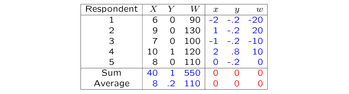
Average:
Deviation score:
Variance & standard deviation
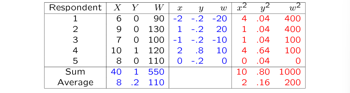
Variance:
Standard deviation:
⭐we are only gonna use for this course, not → NO !
Standardized scores ( - scores)
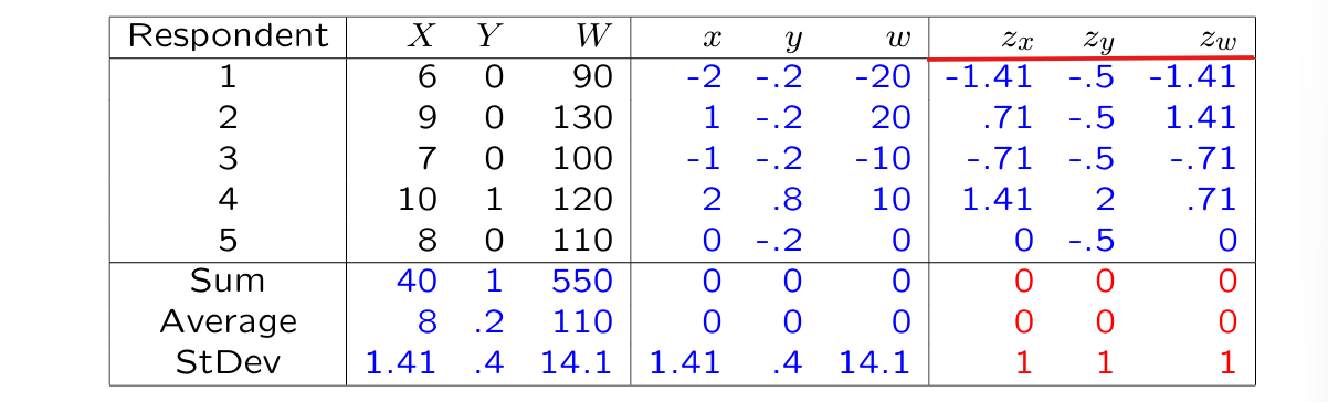
- score:
Covariance & correlation
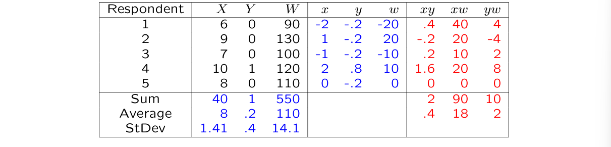
covariance:
S_{XW} = 18

variance-covariance matrix:
⭐diagonal → variance (check)
⭐off-diagonal → covariance
Correlation:
correlation matrix:

⭐diagonal → always 1 (they correlate with themselves)
⭐off-diagonal → correlations
L2 - PROPRTIES OF TESTS & ITEMS
properties of items & tests
What is a Psychological Test?
Cronbach (1960): “a systematic procedure for comparing the behavior of two or more people”
this “procedure” can take on many forms:
multiple-choice aptitude test
personality test with open-ended questions
systematic behavioral observation
Rorschach inkblot test
3 crucial properties:
aimed at measuring behavior (observable)
systematic (objective)
comparison of different people (comparative)
Type of Tests
tests for maximum performance vs typical performance:
maximum performance tests for measuring skills/aptitude
typical performance tests for measuring personality traits, attitudes, disorders…
few differences in statistical analysis of tests scores
2 types of maximum performance tests:
power tests
measure skill without time pressure (most common)
more skilled people give more correct answers
speed tests
measure skill under severe time pressure
question difficulty is trivial
more skilled people answer more questions within the time limit
Bourdon dot concentration test (speed test)
one of the oldest psychological tests
quickly tick the ones that have 4 dots
useful for train conductors, so they don’t run people over
speed - cognitive psychology
norm-referenced or criterion-referenced tests:
norm-referenced tests
compare people to the rest of the population
good norm data on this population of great importance
criterion-referenced tests
compare people with an absolute standard
test inferences are NOT tied to performance level in the population
test theory exam
What Does a Psychological Test Contain?
test material → stimuli / questions
test forms → registering the results (circling answer sheet)
test manual
definitions
precise tests instructions
score-processing procedure
norm tables
discussion of scientific qualities
Example test material
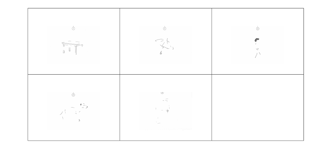
Example test form
Item | Answer | Score X |
1 | table | 1 |
2 | umbrella | 1 |
3 | ? | 0 |
4… | cat | 0 |
…22 | door | 1 |
test score X | 3 |
the step answer to score is the assessment
item scores are determined such that they are indicative of the construct you want to measure: higher item scores = “higher” on that attribute
maximum test: this is fine
but in performance tests we have contra-indicative questions → you need to invert their scores (extraversion tests also has introversion questions)
Properties of the Test Score
test score is generally the sum of the item scores
most important outcome of the test that is used
test manual gives instructions on how to interpret the score (L3)
with norm-referenced tests, norm table needs to be consulted
e.g., 30% of boys aged 3 have a score lower than 3 (30th percentile)
Measurement Level Test Score
test score is a number
interpretation of this number depends on the level of measurement of the test score:
nominal (personality tests)
ordinal (short likert scales) → almost all psychological tests
interval (long likert scales) → equal intervals, no 0
ratio (bourdon dot test) → equal intervals, has a true 0 (not often used in psychology, no 0 level of extraversion)
Test scores with interval level of measurement?
scores are only of interval (or ratio) level of measurement if they are “quantitative”:
an increase of 1 score point always need to reflect the same specific increase in the property you are measuring
Person A,B, and C with introversion scores 10,20, and 30
score difference between A & B and between B & C are equal
not obvious that differences in introversion are comparable!
test scores are (usually) the sum of item scores
item scores are evidently ordinal
test scores therefore formally also ordinal
for practical/statistical purposes we often act as if the test scores are on the interval level of measurement
only justifiable for long tests with a wide range of scores
Variation as Desirable Property
test score intended to reveal differences between people
only possible if people differ in their test scores
High degree of variation in test scores is desirable
Because the test score is constructed out of item scores:
High variance on item scores also desirable
High covariance between item scores desirable
Variation of Test Scores
E.g.: Test score constructed out of item scores and
What influences the test score-variance ?
Test-score variance goes up as item-score variance increases
Quality check items: enough variance?
Correlation between items also of importance:
Some people score high on almost all items
Some people score low on almost all items
This increases variation in the test scores
Preliminary Study of Multiple-choice items
MC items dichotomous scoring: correct = 1, wrong = 0
-value of an item denotes the proportion of correct answers
Unfortunately the same term as with significance tests, but it has a different meaning!
= average item score
is proportion incorrect answers on an item
Ideally , because then item score-variance is maximized
Example multiple choice
Which state does not belong to the USA?
a) New Mexico
b) Washington
c) Ontario
d) Kentucky
Item response is the selected option from a, b, c, d
People that choose c receive an item score of 1
People that choose a, b, or d receive an item score of 0
frequency of use of each answer option gives insight into how an item functions
-value: proportion of people that choose a specific wrong alternative

( in this example)
because people that do not know the answer can guess:
the -value should be higher than every -value
ideally all wrong options (= distractors) chosen equally often:
ideally high item-score variance, which we reach if
Example preliminary study of MC items
which items function properly?

item 1:
-value > every -value
item 2:
-value > every -value
item 3:
-value > every -value
→ ⭐94% got it right - low variance
item 4:
-value > every -value
Preliminary Study of Polytomous Items
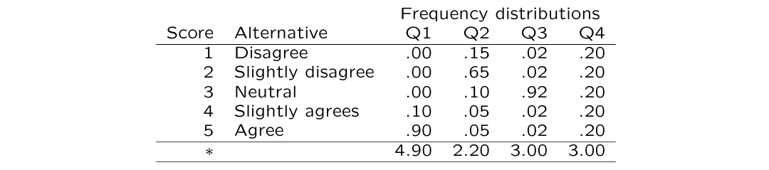
likert → no -value because no right or wrong
if this was a maximum test there would be a correct answer
Q1= ‘Popular’ item; little variation
Q2= Somewhat unpopular item; OK variation
Q3= Neutral item; little variation
Q4= Neutral item; a lot of variation (ideal!)
Preliminary Study: Objectivity of the Test
Test score needs to be determined as objectively as possible
Easy for MC items, but not for other types of items
Assessing open-ended questions
Behavioral observations
Rorschach inkblot test
Different assessors can differ in how they code answers/behavior
Objectivity: Inter-rater reliability
Different assessors/test givers need to draw the same conclusions as much as possible
Extent of agreement between judgements of different assessors needs to be as high as possible:
Inter-rater reliability
Correlation between test scores of different assessors
For test scores of interval level → correlation
For nominal or ordinal level → Cohen’s kappa
Objectivity: Cohen’s Kappa
Kappa determines agreement in categorization of 2 assessors
value 1 → perfect agreement
value 0 → agreement at chance level
example: assignment 60 internships to 100 students
some assessors will select the same category purely based on coincidence
Kappa corrects for this chance
→ proportion of agreement
→ agreement expected due to chance
e.g.: assessors A and B both randomly select 60 students for an internship

of the cases assessors agreed
but what is ? what is the proportion of agreement you would expect based on chance?
both A and B decline of the cases
both A and B accept of the cases
you expect in of cases that both decline
and in of cases that both accept
→
therefore in this case
amount of observed agreement is equal to what is expected based on coincidence
Kappa can also be calculated for three or more categories
example:
3 grades (insufficient, sufficient, good)
50 students
2 assessors (A & B)
to what extent do the teachers’ judgement match?
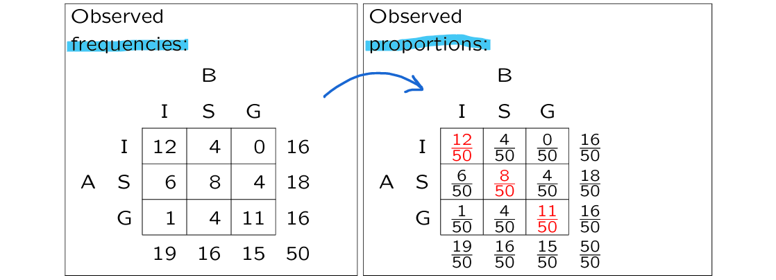
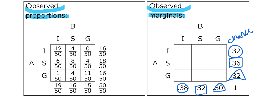
we need the expected proportion of people on the diagonal
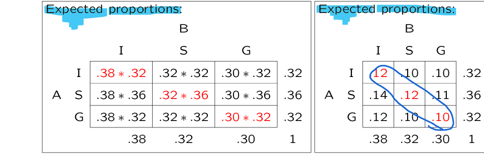
expected proportion is calculated by multiplying the marginal proportion of assessor A with that of assessor B
(careful with rounding !!!)
in % of cases teachers did agree
purely by chance we expect them to agree in % of cases
only modest agreement between teachers
Kappa should be closer to 1 for high-stake tests (at least .7)
L3 - TRANSFORMED SCORES & NORMS
processing tests scores
Transformed Scores & Norms
1) Comparison with an absolute standard
2) Comparison of norms based on ranking
Intermezzo: Linear transformations
3) Comparison of norms based on average and variation
Transformation of Standard Scores
Non-linear
Overview of All Transformations (nonlinear in blue)
L3:
p3
6 points
p4
norm reference and criterion reference tests from last lecture
norm reference have normative character but criterion don’t
p5
it’s not norm reference because it is an objective criteria
p6
continuous: percentile = who is on your left side
ordinal /categorical data: percentile = 1-2 → 0.5-2.5 we look at cumulative scores lower than you
p7
1.4% people have 2 or lower scores
1=0.7
2=1.4 (1+2)
1.4 - 0.7 → just score 2
p8
yellow slides are things you should have seen before
p9
correlation stays the same with linear transformation
if b is negative (usually isn’t ) than the sign of the correlation changes
p11
but not all linear distributions are normal distributions
watch lecture
p13
non-linear transformation → we change the shape
p16
psychologists use this because people clients like to hear more “logical” scores
KNOW THESE THREE RULES!!!!!!!!!!!!!!!!!!!
p17
to get whole numbers
L4 -
L4
p8
systematic part stays the same across the tests
p9
most important formula of the course
t - systematic part - true score
e - random part
p10
black - things that we OBSERVE
red - actually unknown
Nuis - X11 X12 X13…
Verbij - X21 X22 X23…
p11
T - average of scores
p12
average error is 0 because it cancels out
standard error (standard deviation of the error)
standard error = standard observed score
p13
we switched to using one test on multiple people (before this we were testing the same people multiple times)
we find the red numbers by these assumptions
rEY - y can be anything
Error is random so it shouldn’t be predicted by anything
we will never get a true score - we never observe - we can make an inference about it
p14
RXX - X’s mean different replications of the same test
or RXX’
READ THE BOOK ABOUT OTHER DEFINITIONS THAN 5.5
R is red - no one can know the actual reliability
reliability is about
p18
lower reliability → wider interval
L5 -
L5
p4
higher relibility = lower standard error
situation 1
based on the CI s we have way too much overlap because the test is unreliable
situation 2
no overlap, the test is more relaible
p5
reliability is usually assessed by at least 2 tests however internal consistency method only uses 1 test
p6
no serious psychologist should use test-retest methods
p7
T is the same across the two tests → scores are interchangeable
standard error (?) is also the same across tests
p8
essentialy test retest methods without the memory effects
p9
if i standardize both tests i satisfy A and B
and we can standardize these tests because linear transformation doesn’t make you lose data
C look for correlations with other relevant tests on both tests individually
parallel is also not really useful in psychology
p10
set of methods (over a 100 methods) we are gonna look at 4 of them
p15
second most important formula in this course
first is X = T+ E
cii’ → c is covariance, i is one item, i’ is another number
p18
alpha 0.85 and reliability 0.90
we know that the reliability line is to the right of the alpha
so alpha <_ Rxx
the larger the sample the smaller the variance
p22
KR20 = alpha just an easier way to calculate
p25
intervals must be equal
u need a difference of 8 points to compare scores
7 and 15
p28
4 out of 6
16 out of 24
we are still bettwer off because standard deviation went 4 points higher
but standard error only went up less than 2 points
L6 -
L6
p4
k - items
2.8 wrong
p5
we mostly use raw a
p6
test score variance is a good thing
we are interested in differences in people var makes that easier
p8
for multidimension - don’t use raw alpha
p9
ic - internal consistency like raw/normal a
p11
s2x = full tests var - not .8 (p10) but 1.6
usually there is no 0 on the matrix so u need to add everything for s2x
p13
n - lengthening factor
all items need to be parallel (interchangeable, same quality)
p15
the more reliable your test the slower the reliability will increase
p17
never round down like you usually would
p20
d - our new variable
L7 -
L7
p3
discrimination is a good thing in test theory
p5
we need a good rest score
formula: we add every score except for the item we are interested in
SPSS
kick items ur not interested
keep “alpha” as default
options or statistics → check “scale if deleted”
p6
red ones are below 3
we remove them
p9
scores → low to high
draw the line between 7 and 8
p10
bold are the highest so they are selected
p15
attentuation of correlations - weaker correlations
L8 - CONSTRUCT VALIDITY (CH8&9)
test-quality assessment (validity)
(Construct) Validity & Reliability
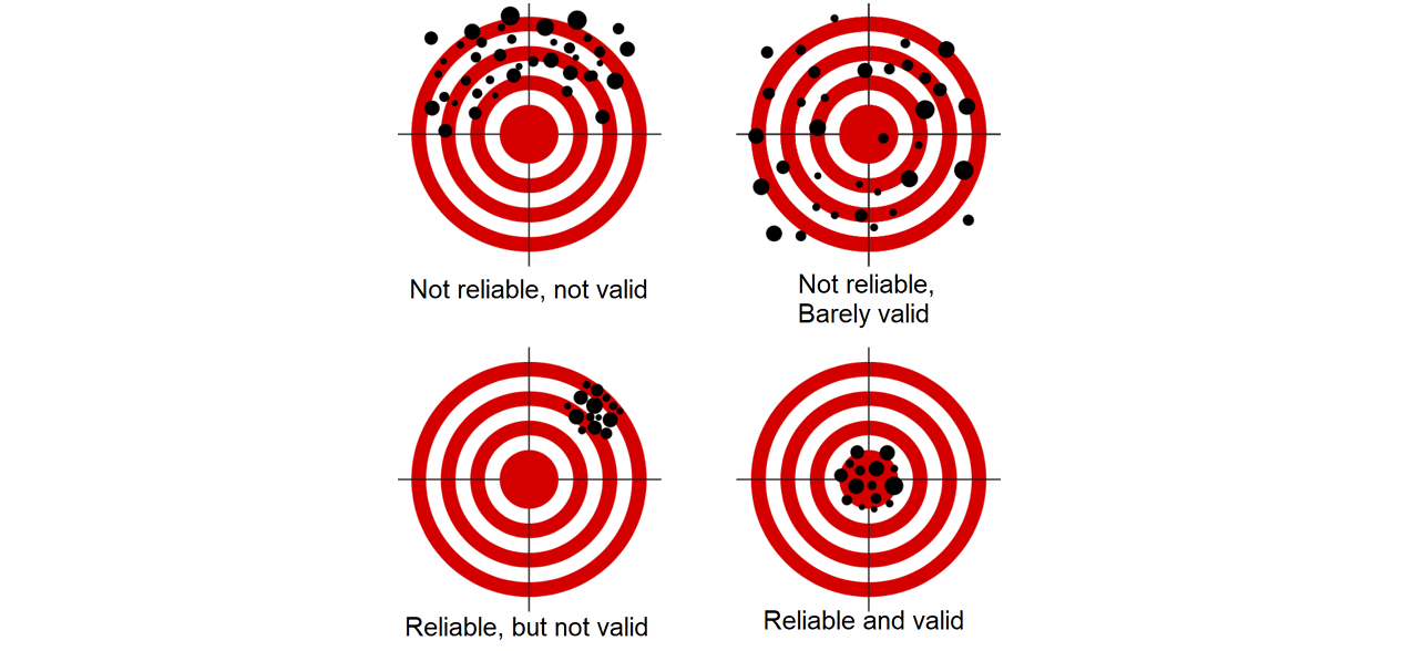
⭐you cannot have validity without reliability
top left: people can make themselves look more extraverted if they know that it’s desired → social desirability bias (construct validity)
The Concept of Validity
many different definitions of validity exists, but most important general definition:
validity: degree to which a test serves it’s purpose
validity depends on the purpose
use of test can be valid, a test itself cannot be valid
a good IQ test won’t be valid if you try to assess depression with it
or if a test was made for a specific population it won’t be valid when given to a different population
when do we conclude that a test performs sufficiently well?
Two Kinds of Validity
1. Construct validity (this lecture)
to what extent is the “hypothetical construct” responsible for the test score? → psychological meaning
what exactly does my test measure?
focal point within scientific research
2. Criterion validity (next lecture)
also called predictive validity
how well does a test predict behavior or performance outside of the test? → criterion in present, past, or future
can I use my test to predict something else?
focal point for practical use test
⭐construct validity and criterion validity are related!
Relationship Construct & Criterion Validity
without construct validity no criterion validity
only reason that the test predicts something is because it measures something relevant
without criterion validity no construct validity
if the test measures something relevant it also should be able to predict something
some psychologists see criterion validity as one aspect of construct validity BUT separating the two validities is more convenient
Pentagon of Construct Validity (fig. 8.1)
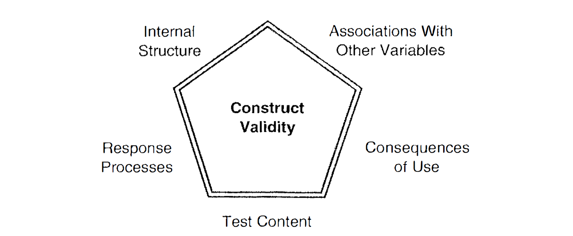
Pentagon of construct validity indicates what we need to pay attention to when determining construct validity of a test:
1. Content of a test
2. Association of test components
3. Response processes
4. Consequences of test use
5. Association with other constructs
5 Aspects of Construct Validity
Pentagon of construct validity indicates what we need to pay attention to when determining construct validity of a test:
1) Content of a test
⭐is about content validity
content of items should relate to the construct you want to measure
content of items should NOT relate to any other constructs → bachelor thesis: many fail
paragraph math questions also assess language
set of items together need to sufficiently cover the constructs → bachelor thesis: many fail
all important aspects of the construct need to be covered sufficiently
balance needs to be in order
IQ test that has only special reasoning
Content validity vs Face validity
face validity relates to content validity
face validity → content validity as assessed by laymen
not important for psychometric quality of the test (because the laymen is not an expert)
sometimes important for practical use:
results of test with low face validity are accepted less often in practice
for example: in NL people rioted against a math exam because they thought it didn’t measure effectively, even though it did (it had high content validity but low face validity)
⭐good content validity usually leads to face validity, but NOT the other way around!
2) Association of test components
if all items measure the same property we expect a “positive manifold”:
positive manifold: positive correlations between all items
important for both the reliability of the test (L6) as well as the validity
we often want a unidimensional test
multidimensional test also possible, if it relates to theory (point 1)
for multidimensional tests: dimensionality of the test is examined by using Factor Analysis
factor analysis is discussed in YEAR 3
read the text about this in CH8, but this is not exam material
⭐examining dimensionality of a test is crucial for (construct) validating the test
unexpected multidimensionality could be at the expense of fairness (point 4 and L12)
⭐internal consistency coefficients like Cronbach’s alpha do NOT give an indication of the number of dimensions
therefore you can’t use it for validity, but only for reliability
we used them to assess reliability only in UNIDIMENSIONAL tests
examining association between items of extra importance for multidimensional tests (e.g. you don’t expect spatial reasoning and logical reasoning to have a high correlation)
multidimensional tests often work with related “subconstructs”
example: related to different aspects of intelligence (RAKIT)
does every item measure its intended subconstruct?
do the items measure other subconstructs beyond the intended one?
⭐key point:do individual items measure what they need to measure?
3) Response processes
Response processes for maximum-performance tests
items are formulated to elicit certain response processes
maximum-performance test:
maximum effort to solve problem
often a certain intended path towards the solution
following the right path leads to the correct answer
⭐if these assumptions are violated it will be at the expense of the validity of the measurement
» Maximum effort to solve problem
assumption is that on a maximum-performance test everybody puts in maximum effort
in that case the performance hopefully gives a good indication of what you’re capable of
if everybody doesn’t put maximum effort this will be at the expense of the validity of the measurement
some people will score low because they are not skilled
some people score low because they have low motivation
possible to examine partly with“process data” → e.g. response times!
» One path to the solution
performances are comparable ONLY if people try to do the same thing (= go through the same response processes)
For example: solving 17×99
respondent A uses multiplication rules
respondent B solves this by 17×100 - 17
respondent C has memorized all the multiplication tables and knows the answer
→ we are NOT measuring the same skill for everyone!
» Multiple solutions possible?
item aims to measure the same construct as the rest of the test
more skilled respondents should always have a higher chance to solve an item correctly
→ problematic if there are multiple solutions (or if the wrong option is also counted as correct one)
we can detect this by using:
discrimination-index D (L7)
item-response theory analyses (L10 & 11)
Response processes for typical-performance tests
typical-performance items meant to gain insight into someone’s “true” attitude or personality
in practice many response styles can threaten validity:
social desirability
acquiescence
extreme vs mild answer tendency
distorts the measurement of the intended property!
» Response style 1: Social desirability
In theory for typical performance items no right or wrong answers
BUT in practice some answers are more desirable:
Positive image of yourself towards others
Positive image of yourself towards yourself!
Respondents can take this into account in their answering behavioSocial desirability tests (“I never lie” → obviously a lie) exist, but correction is difficult
Anti-social response style (= provoking) also possible
» Response style 2: Acquiescence
tendency to agree → some people have a tendency to agree with statements rather than disagree (sometimes because of culture)
social desirability (otherwise disagreeing with the researcher)
cognitive biases
causes measurement to be distorted
if only indicative items — acquiescence → overestimation
solution: balance indicative and contra-indicative items
» Response style 3: Extreme vs mild response style
some people are quick to claim an extreme position
for Likert, they often pick the most extreme options
leads to overestimation of extremeness of their position / personality
counterpart: mild response style
people choose the neutral option independent of content
→ solution: advanced statistical methods
also measure response style with the test
CANNOT with
classical test theory frameworks(everything we saw till now)we can with item-response theory(next week)
4) Consequences of test use on validity
validity: degree to which a test serves its purpose
validity is NOT separate from how the test is used
improper or unfair use of test → not valid
debatable whether this should fall under construct validity
improper use could be the users fault
problem is in this case not the measurement itself, but what’s done with it
5) Association with other constructs
construct validity is about the question to what extent the test measures the construct of interest
from psychological theory we know how this constructs relates to other constructs
for example, intelligence should be associated with school performance
association between constructs and their corresponding tests captured in a nomological network
then you examine if the scores on the test are also correlated with these constructs
empirical validation research
⭐not seeing the associations that should be there is just as problematic as seeing associations that shouldn’t be there
Empirically researching nomological network
if the test measures what it is supposed to measure, then the test score…
correlates strongly with scores on tests that measure the same construct (= convergent validity*)
correlates with scores on tests that measure related constructs (= convergent validity)
does NOT correlate with scores on tests that measure unrelated constructs (= discriminant validity)
here we do assume that the other tests are reliable and valid!
resembles criterion validity, but now there is no emphasis on any particular criterion
Nomological network GLT & study skills
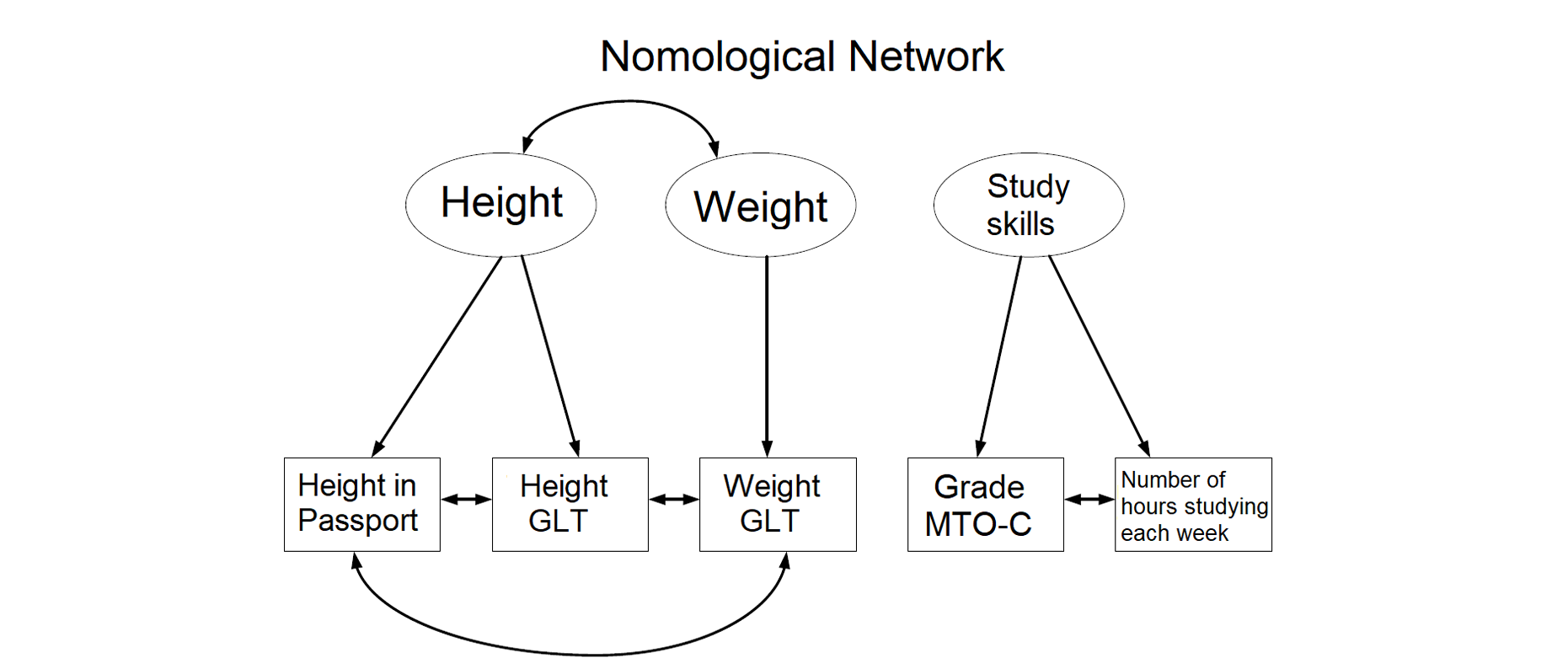
Convergent validity GLT
Examining association between tests that measure the same thing (using simple linear regression)

→ our test predicts height, as intended = pass
examining association between test that measure related constructs

→ lower correlation than height = pass
Discriminant validity GLT+
examining association between test that measure unrelated constructs

→ not correlated =pass
Multitrait-multimethod research
systematic research on convergent and discriminant validity using Multitrait-multimethod research
research on multiple constructs (= Multitrait)
every “trait” is measured using multiple methods (= multimethod)
correlation between every trait-method combination with every other combination is determined
EXAMPLE: MTMM RESEARCH
measuring of three personality traits for school children:
friendliness (T-F)
tidiness (T-T)
dominance (T-D)
three measurement methods (= types of tests) investigated:
self-assessment (M-S)
peer-assessment (M-P)
teacher’s judgement (M-T)
3×3 = 9 trait-method combinations (therefore 9 tests)
every pair of those 9 tests is examined (correlation)
you hope to find…
high correlation between measurements of the same constructs based on different methods → convergent validity
low correlation between measurements of different constructs based on different methods → discriminant validity
low correlation between measurement of different constructs based on the same methods → discriminant validity & ✨absence of method effects✨
method effects:
association between measurements of unrelated constructs due to the fact that the same measurement method has been used
undesirable, because the constructs are not correlated
results in spurious correlations
finally: reliability of every test is placed on the diagonal table ↴
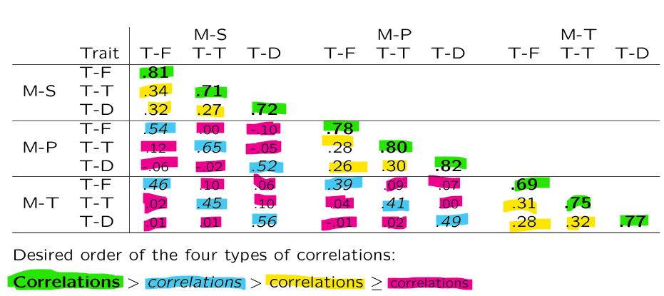
⭐method effects:
M-T x M-S (different methods) → T-D and T-F have a r = .01
BUT M-S x M-S (same method) → T-D and T-F have a r = .32.
⭐big diagonal (bold ones) = reliability
L9 - CRITERION VALIDITY (CH9)
test-quality assessment (validity)
Using a Test in Practice
test can be reliable and have good construct validity
does NOT yet tell us whether or not the test is practically relevant!
can we use the test to make predictions about whether the examined persons (will) satisfy a certain relevant criterion?
does the use of the test add to the quality of the decisions we take about these persons?
→ this is the question of criterion validity
Logic of Using Tests for Decisions
often we want to take decisions using a criterion that is not available
often it’s impossible to measure the criterion before you have made the decision
study success criterion for admission to school
effect of psychological treatment on depressed client
you want to know before someone commits suicide, so you can prevent
by measuring a relevant property you hope to predict the criterion
test function as “stand-in” for the not observed criterion
of course not exactly the same (correlation < 1):
if we take a decision based on the test score instead of the not observed criterion our decision becomes worse
is a decision based on the test score better than a decision without this test score? and how much better?
degree to which the test score helps with making the correct decision will depend on the association between the test scores and the criterion
Examining Criterion Validity
criterion validity is determined by the association between test score and criterion
normally the criterion will not be available when you make the decision
determining criterion validity requires dedicated research:
large and representative sample
everyone takes the test
criterion is measured (later) for everyone as well
if both test score as well as criterion are determined you can study the validity
first step is examining the correlation between the two scores ()
→ test is perfect stand-in for criterion!
→ test is completely unrelated to criterion (does not add anything to decision making process)
this correlation is often called predictive validity (= criterion validity)
Predictive Validity in Practice
in practice low correlation is often found between test score and criterion
estimated correlation is influenced by:
Restriction of range for test score(= design error research!)
Restriction of range for criterion
Non-linear association test score and criterion
Heteroscedasticity
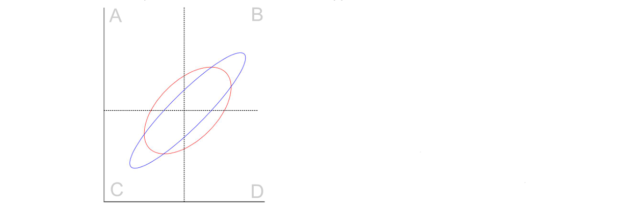
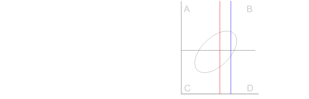
1) Restriction of range for the test score
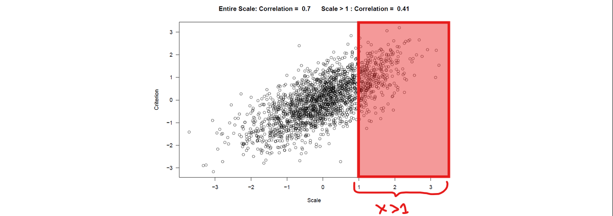
Admitted group (X>1 ) is more homogenous than the group as a whole → lower estimated correlation
2) Restriction of range for the criterion
same problem can also play a role for the criterion
not everyone that the test was administered to is available later on to measure the criterion
if attrition depends on the criterion it distorts the image!
often occurs with selection tests: poorly performing individuals don’t “survive” until the moment criterion is measured
here it is also the case that the remaining group is more homogenous than the group as a whole → lower correlation
»1&2) Restriction on both test score and criterion
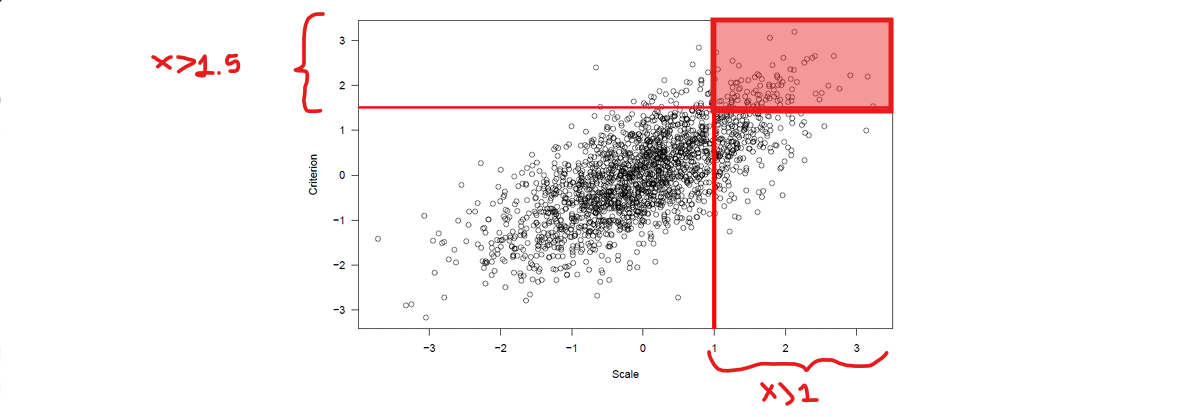
remaining group (Y>1.5 ) & (X>1) is even more homogenous than the group that we selected (X>1) → estimated correlation practically
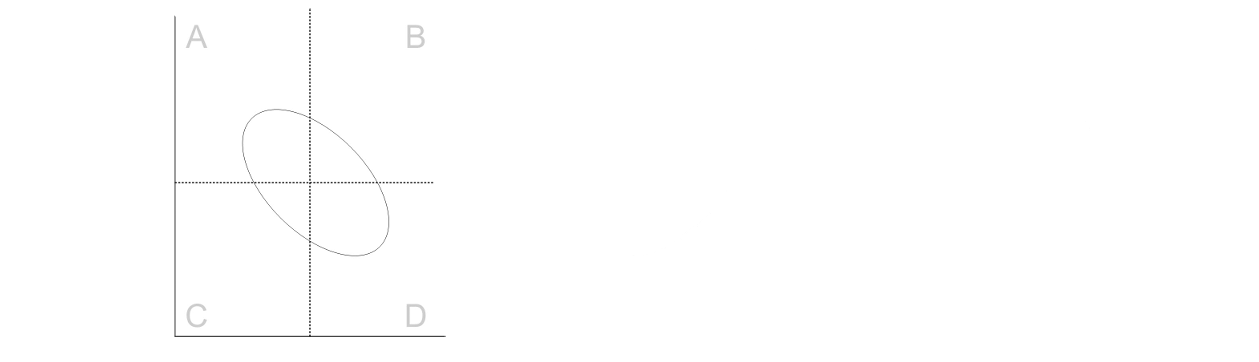
3) Non-linear association test score and criterion
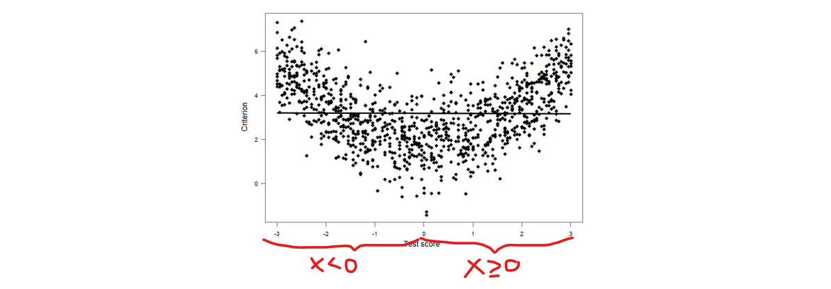
strength and direction of the association between and criterion now depends on the test score:
X<0 →
→
⭐there is a relationship, just not linear → test score does predict the criterion. However, the overall correlations is still 0.
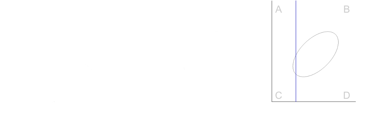
4) Heteroscedasticity (unequal variance)
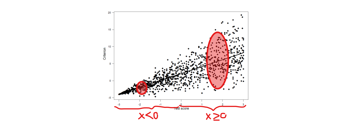
strength association between test score and criterion now depends on the test score:
X<0 →
→
⭐for example, to hire people for OpenAI the company is using a test to measure applicant’s programming skills
→ all people who scored low on the test (X) will also be bad at the job (Y) = low variance
→ not everyone who scored high on the test (X) will be good at the job (Y) = high variance
→ this is a good test to filter out people who are definitely not going to make it, but a bad test for figuring out who will do well
Predictive Validity Often Low
even if these 4 problems do not play a role, predictive validity is often low
multiple possible reasons:
Measurement of the criterion is unreliable
Measurement of the criterion is not valid
Reliability & Maximum Predictive Validity
predictive validity is measured by
we still know from L7:
thus low if or is low, even though is high!!!
reliability of measurement of criterion very important, but often overlooked
Validity Criterion Measurement
idea is that the test predicts the actual criterion
if we measure this criterion incorrectly this influences !
can be lower than real association between test score and actual criterion:
intelligence test () possibly good predictor of actual performance ()
but if performance assessment () produces a non-valid measurement of actual performance the correlation will fall short
Criterion Validity for Dichotomous Decisions
tests are often used for making dichotomous decisions
accept / reject
treat / don’t treat
treatment A / treatment B
most important: classify as accurately as possible
not the same as high linear association !
test score is (approximately) continuous:
dichotomous decision based on cutoff score
X<Xcrit → reject (0)
→ accept (1)
the continuous criterion must also be made dichotomous:
Y<Ycrit → does NOT satisfy the criterion
→ does satisfy the criterion
place everyone in a 2 by 2 frequency table!
⭐there’s no optimal critical line, you have to choose whether you prefer false negative or false positive → for example, a false negative is a huge risk considering suicide prevention
Example Criterion Validity & Decisions
students without math background need to pass “Testimonium Mathematics” before start of study
idea is that without this knowledge the chances of successfully studying is low
study success (measured based on credits obtained in year 1 → ) not known at start of study
Test score Testimonium () therefore a “stand-in” for not observed criterion
studying crit, val. only possible after observing criterion
one-time acceptance of all students, regardless of Testimonium score!
year later insight into both Testimonium score and credits
only then insight into validity of the test use:
requires determining criterion limit → here 30 ECTS
does test help for correctly rejecting / accepting students? ↴
Test Use for Dichotomous Decisions
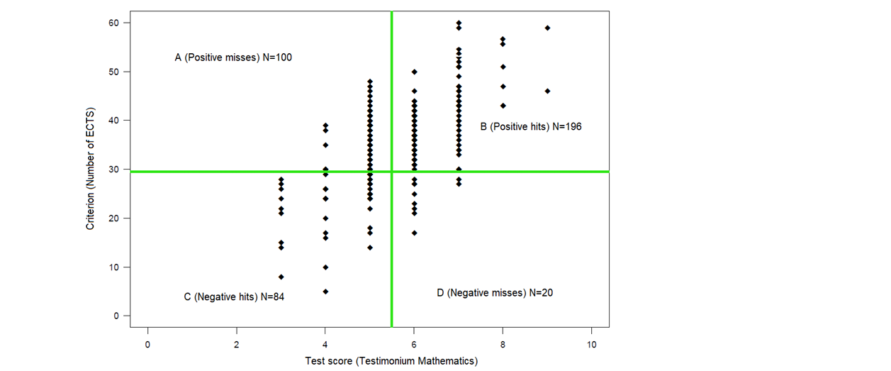
A: positive misses / false negatives (100 students unjustly rejected) → low test score X, high criterion Y
B: positive hits / true positives (196 students justly not rejected) → high test score X and criterion Y
C: negative hits / true negatives (84 students justly rejected) → low test score X and criterion Y
D: negative misses / false positives (20 students unjustly not rejected) → high test score X, low criterion Y
selection rate = proportion accepted students
→
how critical we are with our test → only % will be admitted
⭐selection rate: students accepted based on test score (X) divided by total students
base rate (coincidence) = proportion students who satisfied the criterion
→
coincidence? base rate is what are success rate will be if we don’t use a test → if I admit everyone % will succeed
⭐base rate: students that satisfied the criterion (Y) divided by total students
success rate = of the accepted students, proportion justly accepted
→
needs to be larger than base rate
between the people we accepted, how many were justified → %
⭐success rate: students who satisfied both X and Y divided by all students who satisfied X
sensitivity = of the students satisfying the criterion, proportion that is accepted
→
for example, is people who have Covid and is people who were detected →% of Covid patients were detected by test
needs to be high
⭐sensitivity: students who satisfied both X and Y divided by all students that satisfied Y
specificity = of the students NOT satisfying the criterion, proportion that is rejected
→
how well do we filter out the unsuccessful?
between the people who didn’t satisfy Y, how many did we (correctly) reject → %
⭐specificity: students that did NOT satisfy X and Y divided by all students that did NOT satisfy Y
!!!!!these formulas aren’t on the formula sheet, memorize!!!!!
validity = correlation between dichotomized test and criterion score ( )
⭐same calculation as for determining correlation item score and dichotomized rest score (see L7)!
Criterion↓ | Test → | 0 | 1 | |
1 | 100 (A) | 196 (B) | 296 |
0 | 84 (C) | 20 (D) | 104 |
184 | 216 | 400 |
→ if it’s above 0, it’s doing something: so the success rate will be bigger than the base rate → but is it good enough, depends on our stakes
Success rate / sensitivity dependent on
(1) Validity ()
if larger:
& larger
& smaller
→ success rate ( ): proportion of correctly accepted out of everyone accepted = larger
→ sensitivity (): proportion of accepted out of everyone who satisfied = larger
(2) Selection Rate ()
if we move the further (lowering selection rate / rejecting more people):
& smaller but gets more smaller than → larger compared to
& gets larger
→ success rate ( ): proportion of correctly accepted out of everyone accepted = larger
→ sensitivity (): proportion of accepted out of everyone who satisfied = smaller
⭐you have to choose which one you want to improve!
Success rate / selection rate dependent on
(3) Base Rate ()
large base rate:
larger compared to total
larger compared to
→ success rate ( ): proportion of correctly accepted out of everyone accepted = larger
→ selection rate (): proportion of accepted out of everyone = larger
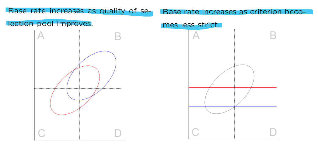
⭐increasing base rate by lowering is usually not feasible though
Remarks for decisions in practice
(1) Problem: many of my hired candidates are unqualified!
cause:
low validity
low base rate (success rate is going to be very low)

high selection rate
(2) Problem: optimal balance positive / negative misses?
depends on the situation:
negative miss / false positive (D): how bad is hiring an unqualified person; treating a non-sick person?
positive miss / false negative (A): how bad is not hiring a qualified person; not treating a sick person?
⭐stricter selection → smaller but larger
⭐more lenient selection → smaller but larger
(3) Relationship success rate, validity, base rate, and selection rate → Taylor-Russel tables
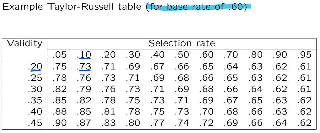
for a base rate of → validity = (low); selection rate = (strict) and Success rate =
why success rate high for a test with low validity?
→ if selection rate is high then the success rate will be closer to base rate: if selection rate is low (in our case) success rate is higher
→ if validity is 0 then success rate = base rate
→ for very large or small base rate: selection rate is pointless
L10 - INTRODUCTION ITEM RESPONSE THEORY watch
advanced use of tests (IRT)
Classical Test Theory
Aimed at reliable measurement ( and )
How to measure a hypothetical construct (e.g. intelligence)?
true score estimated using test score
disadvantages:
(and ) dependent on both respondent and test
if you use a different test the true score changes
we assume: no control over the model (but there is no way to check whether is correct)
Interval measurement level of unverifiable
we assume interval measurement level, but we don’t with if the test score and the construct has the same intervals
1 score higher on the extraversion test doesn’t make you 1 interval higher on extraversion
Implausible assumption: accuracy of the measurement is the same for everyone
people that don’t know much on the exam have a higher variance since they guess the answers
Item Response Theory (IRT)
alternative → Item Response Theory (IRT)
also called Modern Test Theory
→ statistical model for explaining (differences in) item- and test scores based on the hypothetical construct
Beforehand: Models
describe a phenomenon
simplified representation of reality
fit reality to a higher or lesser degree
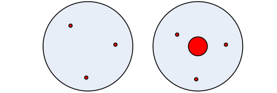
Model of the atom of Thomson (left) & Rutherford (right)
Beforehand: Conditional Probability
MTO (F) | MTO (P) | ||
TT (P) | .40 | .30 (2) (3) | .70 (a) |
TT (F) | .20 | .10 | .30 |
.60 | .40 (1) (b) | 1.0 |
unconditional probability: (MTO = P)
unconditional joint probability: (MTO = P, TT = P)
conditional probability:
3a: (MTO = P | TT = P)
chances of MTO being P given that TT is P
3b: (TT = P | MTO = P)
chances of TT being P given that MTO is P
We saw it before: Item Probabilities for Dichotomous Items
-value (L2): proportion of people that passed the item
this is an unconditional probability!
→ probability that random respondent answers item correctly
But: not everyone has that exact same probability of answering the question correctly!
high-skilled respondents → probability higher than
low-skilled respondents → probability lower than
We saw it before: Item-probabilities & Skill Levels
to determine the discrimination-index we looked at P_{high} and
these are conditional probabilities!
→ probability question correct given respondent belongs to best 30%
respondent in best %
→ probability question correct given respondent belongs to worst 30%
respondent in worst %
problem: the best 30% people still differ among themselves in their probability to correctly answer the item!
we can further split that group up (0-10, 10-20, 20-30)
but they can always be split up further!
what we want is probability of item correct given your exact skill level!
capturing this probability is the focus of Item Response Theory (IRT)
↓
Latent Trait ()
skill level in IRT → theta
often called “latent trait” (not always skill)
E.g., for topographical knowledge
comparable with true score in CTT
everyone has their own value on
E.g. ,
assumption: standard normally distributed (, )
IRT & the Item Characteristic Function
IRT is about determining the probability of correctly answering question given skill level
in other words: what is ( | ) for item and every possible ?
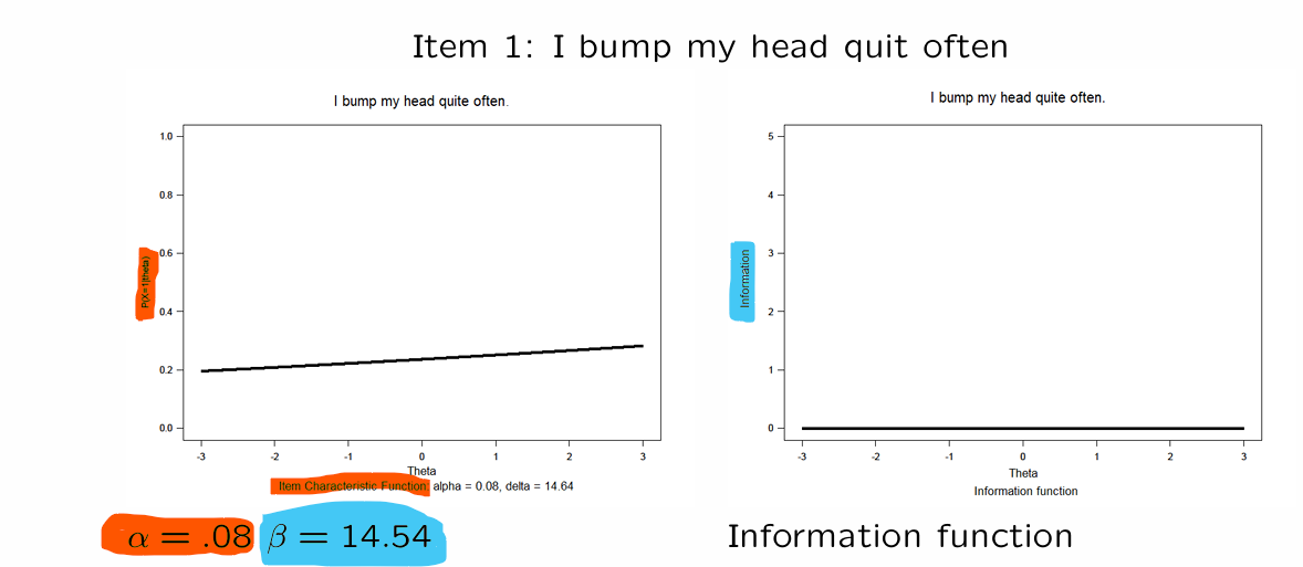
→ this description of the item probability as a function of is called the item characteristic function
item characteristic function shows how much your skill matters for the probability of correctly answering the question
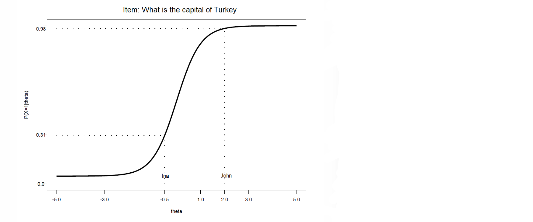
Item characteristic functions
item characteristic function (ICF) different for every item:
NOT all items are equally difficult
NOT all items discriminate equally well
if you know the ICF and , you can determine the probability of answering the question correctly
can be inferred from the figure (later: also calculate)
figure also shows if the item functions well
⭐John knows about geography → his is bigger
⭐therefore, it’s easier for him → his chances of answering correctly is larger
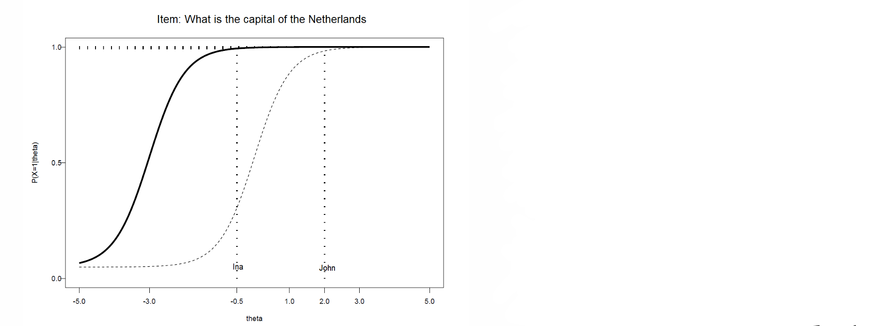
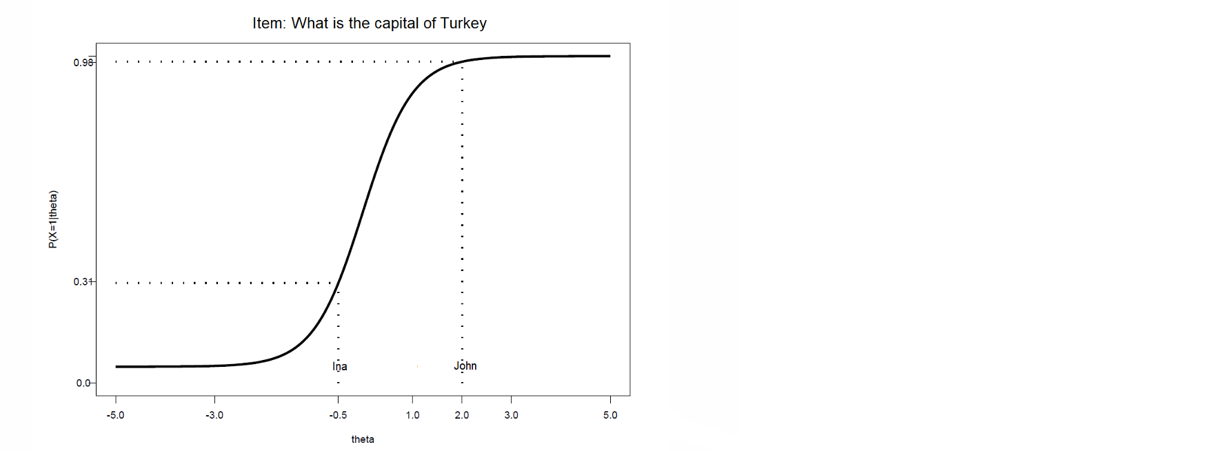
⭐Ina and John are both Dutch, so this is easier than knowing the capital of Turkey → line shifts left but keeps it’s form
⭐But their skill level stays the same, the items difficulty is the only change
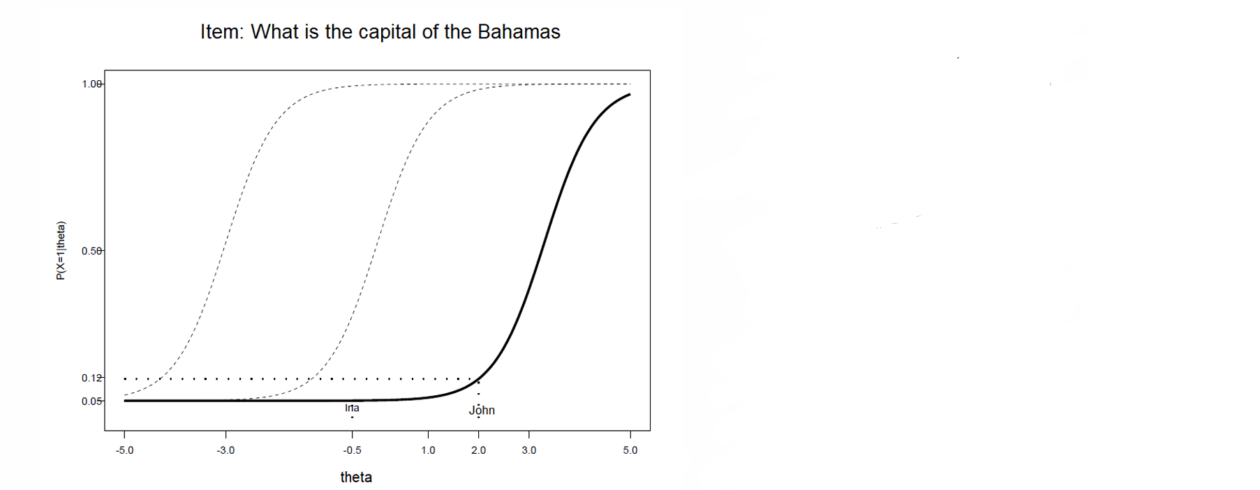
⭐again the skill levels stays the same but the item is harder → line shifts right
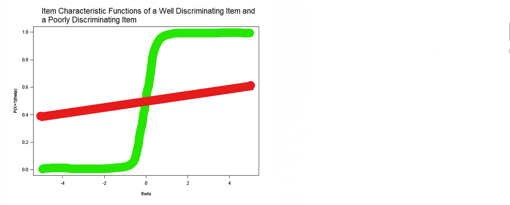
⭐ ( , ) → always in between [0-1] [0-1] → probability!
⭐green → well discriminating
⭐red - poorly discriminating
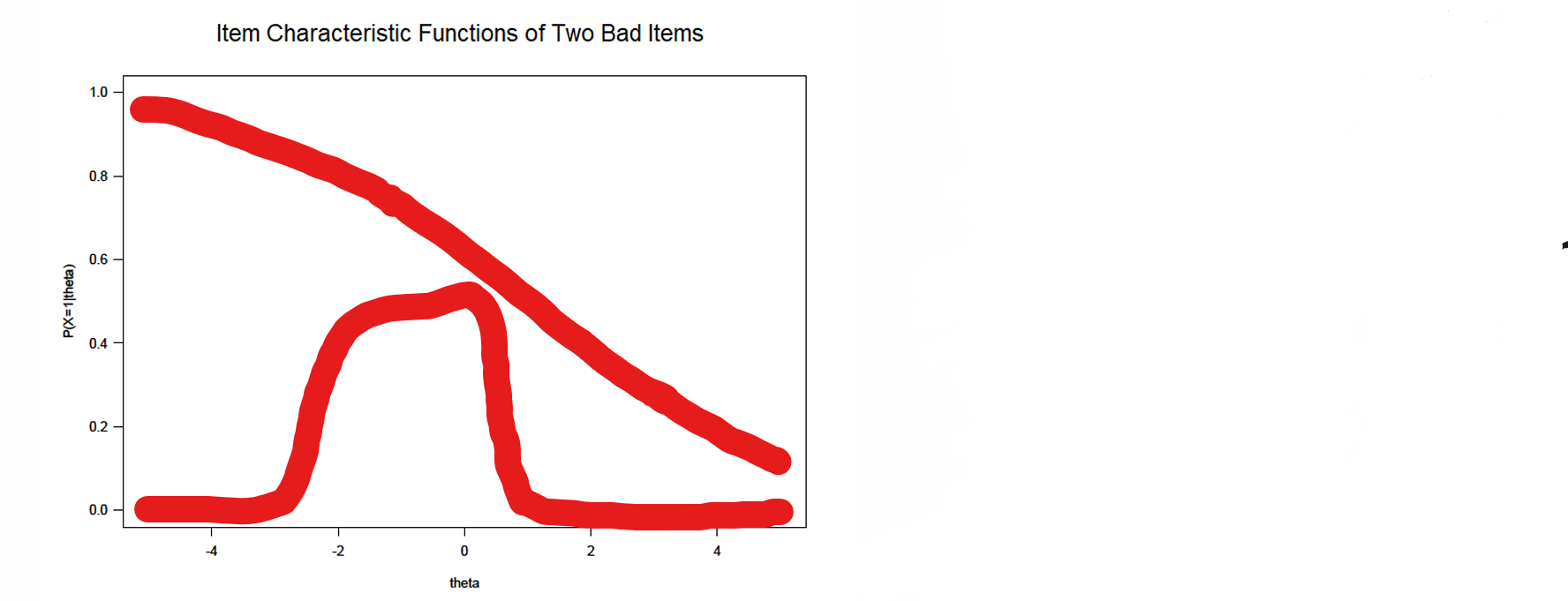
⭐higher skilled people are struggling more → usually recoding error
⭐only average skilled people can answer → the incorrect answer is coded as the right answer
Item characteristic functions & IRT models
how can you determine what the ICF is?
you use an IRT model
model makes assumptions about the shape of the ICF
based on the data you can estimate the ICF for every item
is done by statistical software (not SPSS)
we need to choose an IRT model!
- Exponents
natural logarithm:
exponentiation:
(1+1+1/2 = 2.5)
calculator: exp(3) → 3lnv ln
Logistic Regression for Item-Responses
two IRT models we are gonna learn is literally just logistic regression (you learned in correlational research methods)
⭐these are only for dichotomous tests !!!
(simple) logistic regression is about predicting a dichotomous outcome based on one predictor:
probability of given
Y (DV) and X (IV) can be anything, so we can also fill in:
probability of item given given knowledge
IRT models → logistic regression for item scores
simplest model: Rasch model (set to and rewrite as )
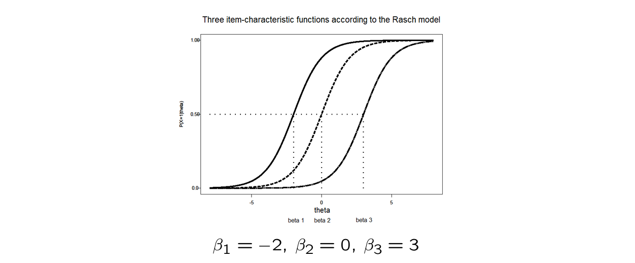
1) Rasch Model = One Parameter Logistic Model
only 1 item parameter: → item difficulty
Rasch model easier to write like this:
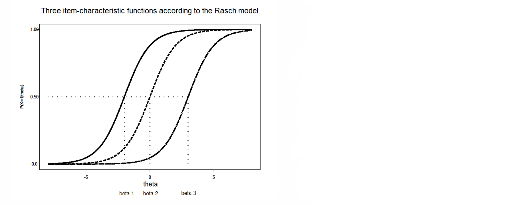
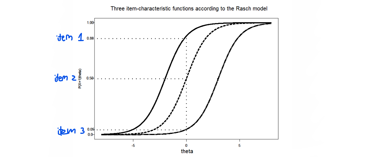
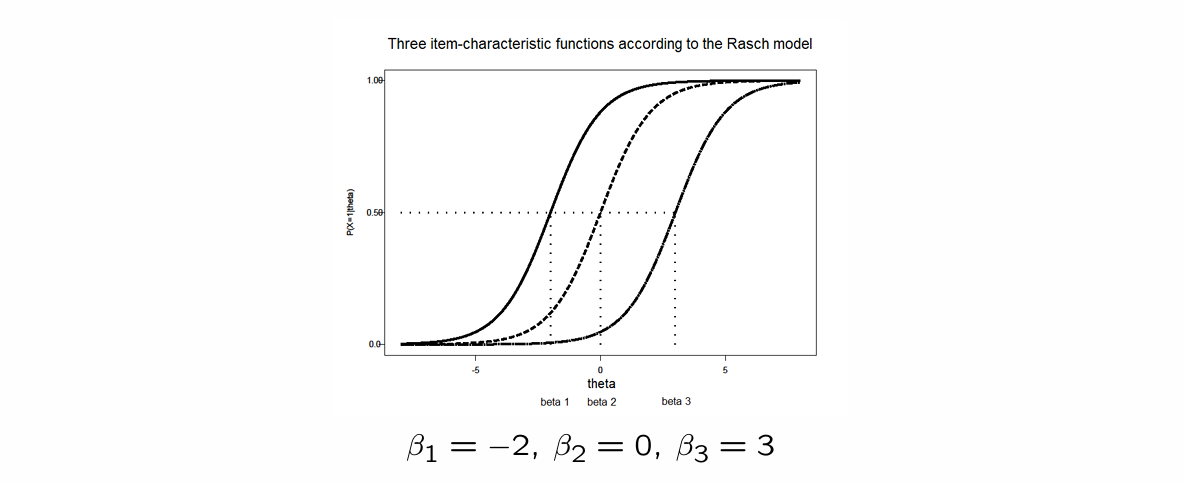
⭐same S curves only the location differs → same discrimination level but difficulty () is different
Rasch model
items can only differ from each other in difficulty ()
ICF looks different for every item
differ only in location of the S-curve
therefore also called location-parameter
: location where for it is the case that:
⭐captures the location you have to be on in order to have % chance of getting it correct
⭐when your ability level () is equal to the item difficulty level ( ) then you have % chance of getting it correct
⭐item location parameter tell us which ability level ( ) you need to have to be at %
Calculations with the Rasch model
imagine a respondent with who answers 3 items with different difficulties:
item 1: fairly easy
item 2: average
item 3: very difficult
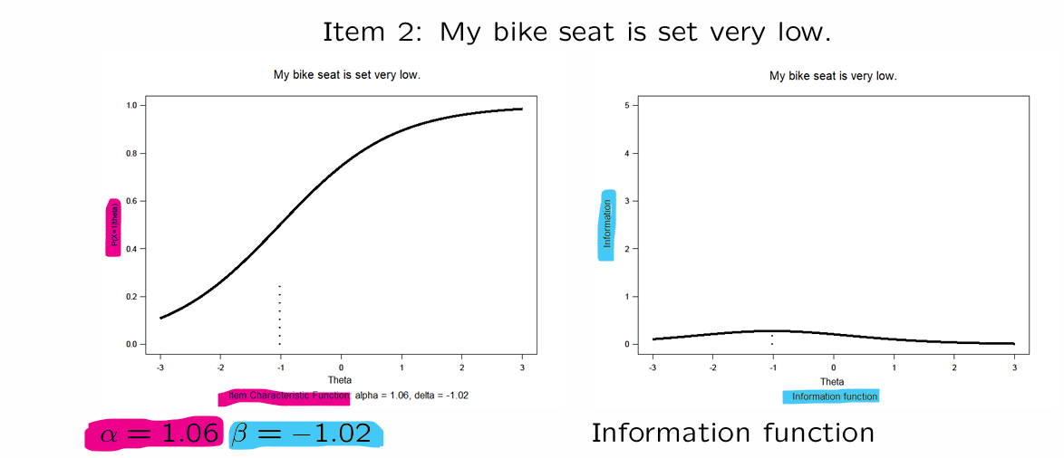
Item-information for Rasch model
Rasch items differ in difficulty
items provide a LOT of information about values close to the item-location ( )
but LITTLE information about values far from there
\theta>>\beta → almost everyone gets question right
\theta<<\beta → almost everyone gets question wrong
ITEM-INFORMATION FUNCTION:
function : if higher → measured more accurately
⭐() → outcome depends on
for example, and…
person A:
person B:
person C:
→ is measured more accurately by the item than the item and

⭐depends on the item-characteristic functions steepness → steeper = more accuracy
Steps IRT Analysis
select your IRT model
draw a large sample from the population
estimate the item-parameters (item-difficulty for Rasch)
then you can use the test to estimate for people
NOT observed, therefore we get an estimate →
3. Estimates of item-parameters Rasch model for GLT data
for item 1: you need to be above average on height to have % chance of saying yes to the item
4. Determining a person’s estimate of
For every person we know which questions they got right/wrong
We have observed their response pattern on the test
Based on the response pattern some values of are more realistic than others
Someone with will not often answer questions with correctly
Software finds the optimal estimate:
number of questions answered correctly (= test score ) determines the estimated
just like CTT: higher X → higher estimated
difference is that we estimate and NOT
concept comparable: more questions correct → higher estimated
most important difference: in IRT standard error of measurement is NOT equal for everyone (L11)
The Model According to Rasch
Population-independence of persons & items
Difficult math test (D) and easy math test (E)
CTT: T_{John,E} > T_{Ina,D} : does not say anything about numeracy of John relative to Ina’s
Rasch model: = ;
Thus we can compare with !
Rasch model: We can also always compare and , even if items and are not in the same test
Strict
Assumption: All functions discriminate to the same degree; no random guessing (same curve shapes)
Therefore: not very flexible item characteristic functions Consequence: model often does not fit!
‘One-parameter logistic model’, because 1 item parameter
Other IRT models are more flexible (= more item parameters), but also more complex
Besides Rasch we only discuss the two-parameter logistic model (2PLM)
Rasch model (one-parameter logistic model)
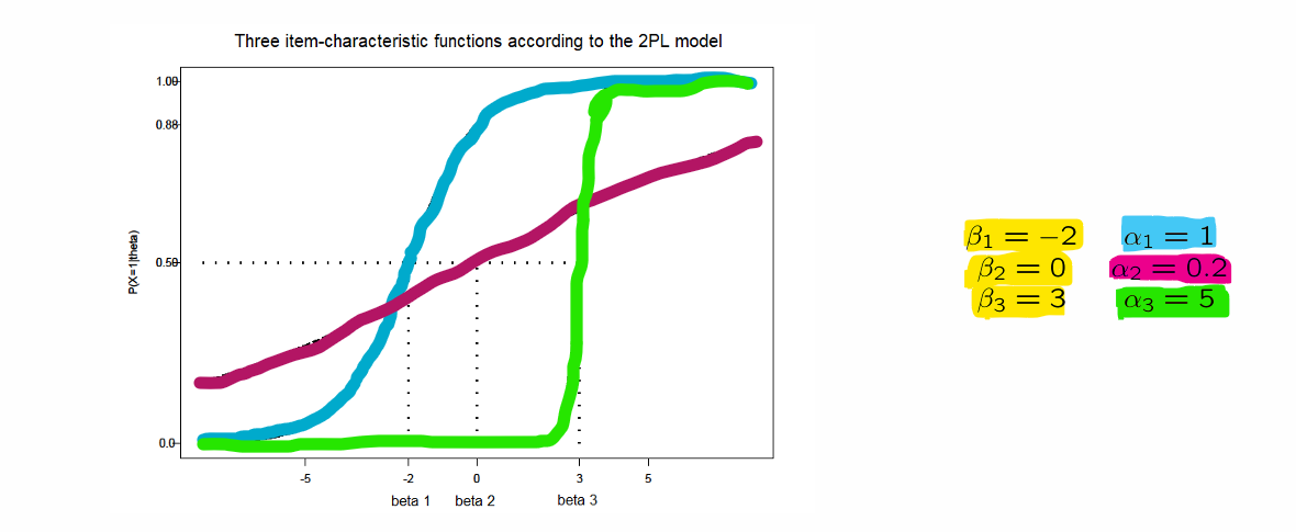
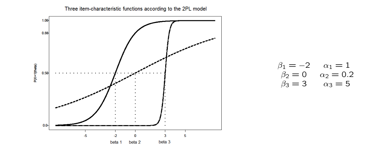
2) Birnbaums Two-parameter (Logistic) Model (2PLM)
Rasch model extended with item-discrimination parameter
indicates how well item i distinguishes between people based on their level on the latent trait
Items now differ in how well they discriminate! However, always the case that α_i > 0
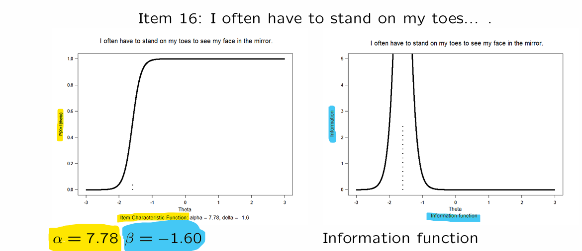
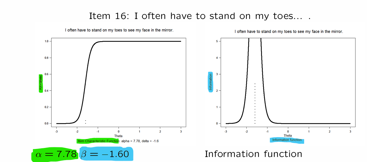
Higher α_i is better; leads to steeper item characteristic functions (= we know more information)
Item-information for 2PLM
2PLM items differ in both difficulty ( ) and discrimination ( )
Similar to Rasch model:
Items provide most information about close to
Different from Rasch model:
Items differ in how well they discriminate
Higher ? → item provides more information!
Birnbaum 2-parameter logistic model
Properties
population-independence
model | persons | items |
CTT | ❌ | ❌ |
Rasch | ✅ | ✅ |
2PLM | ✅ | ❌ |
measurement-level
CTT | unknown (pretend it’s interval) |
Rasch | interval |
2PLM | interval |
Purpose of Item Response Theory
(1) Test construction
estimate item-characteristic functions
select best items
(2) Test administration
estimate for all respondents based on item scores and item-characteristic functions
derive the accuracy with which is estimated
L11 - IRT IN PRACTICE
advanced use of tests (IRT)
Rasch Model (One-parameter Logistic Model)
⭐location → difficulty
Birnbaums Two-Parameter (Logistic) Model (2PLM)
⭐location → difficulty
⭐steepness → discrimination
Purpose of Item Response Theory
(1) Test construction
estimate item-characteristic functions
select best items
(2) Test administration
estimate for all respondents based on item scores and item-characteristic functions
derive the accuracy with which is estimated
Accuracy of Estimation for Different Theories (CTT & IRT)
Accuracy of the estimation of in CTT
estimate from
equal for everyone (assumption)
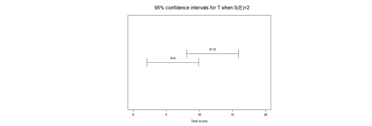
not true! So we need to construct a CI (using )
lower the the more precise our measure (narrower interval)
Since the is the same for everyone CI’s are equally wide, they just differ in location
Not realistic! NOT everyone is measured equally precisely
my test will give us more information about someone than another person
for example, my test might show more variation for people in the low ability range
Accuracy of the estimation of
Item-Information Function : if higher → measured more accurately
⭐() → outcome depends on
for example, and…
person A:
person B:
person C:
→ is measured more accurately by the item than the item and
⭐depends on the item-characteristic functions steepness → steeper = more accuracy
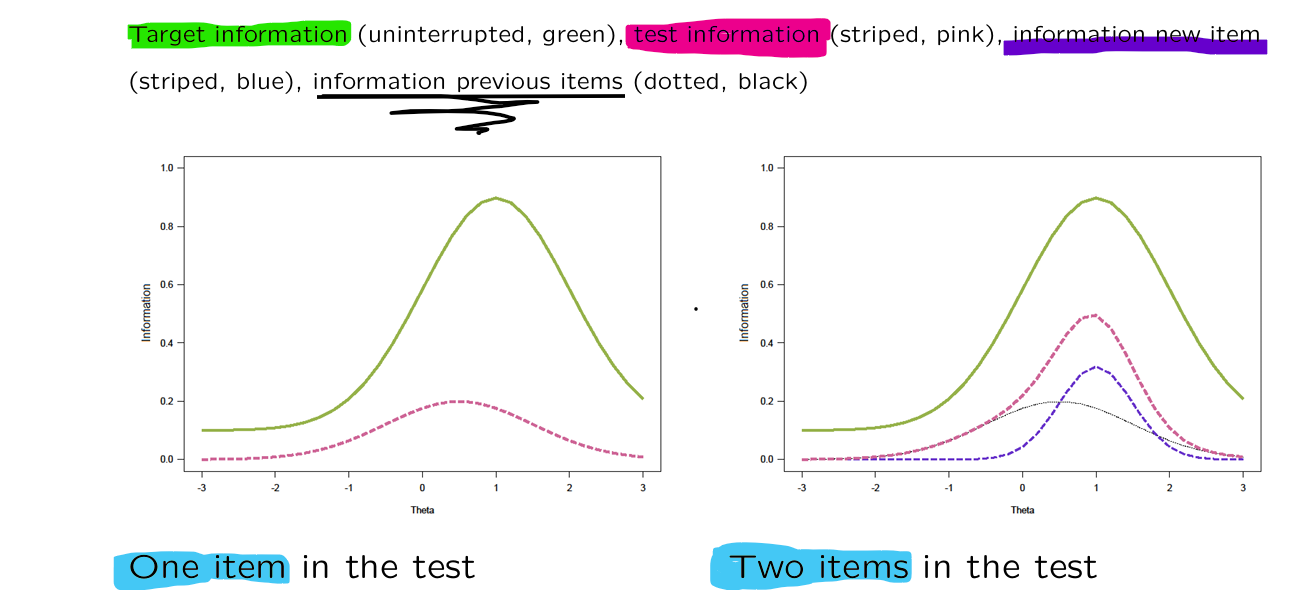
Test Information Function
test information function:
test with 2 Rasch items: and , ,
estimated is more accurate for because it’s the most similar to the ’s → smallest CI interval around estimated

⭐you can get the test information function peak by adding all the peaks of the items
Accuracy of the measurement
standard error of measurement of estimated for the test ( ) is determined by the test information and therefore also depends on !
different values will give us different because NOT everybody is measured equally precisely
⭐() → outcome depends on
95% CI for :
[ ]
⭐the higher the test information for → smaller the CI for that !
Test Construction Based on an Item Bank
item bank: relatively large collection of easily accessible items (ICF and item description known)
elementary math:

you come up with large set of items
give them to al large sample
estimate item-characteristic functions
know you know alpha and beta (also code by different domains)
based on the information you have now,
⭐i can choose different items for 5th graders and 6th graders but i can still compare ’s from different tests
→ what is the desired accuracy of estimated for all different possible values of estimated ?
with IRT population-independent measuring is possible.
With item banks different tests can be composed → depends on the purpose of the test
2 different tests with different purposes:
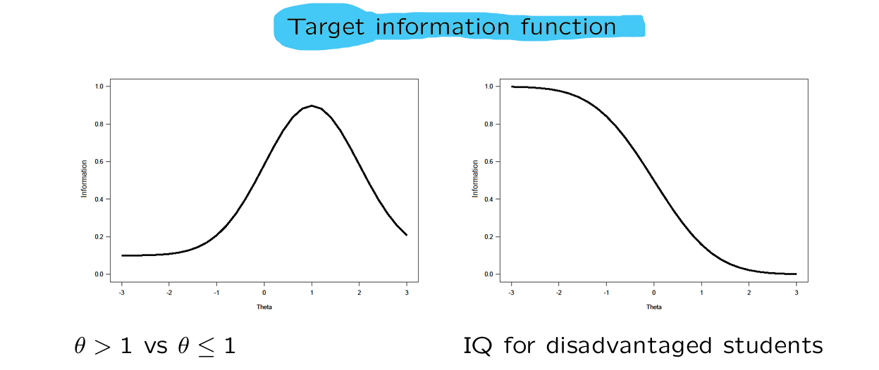
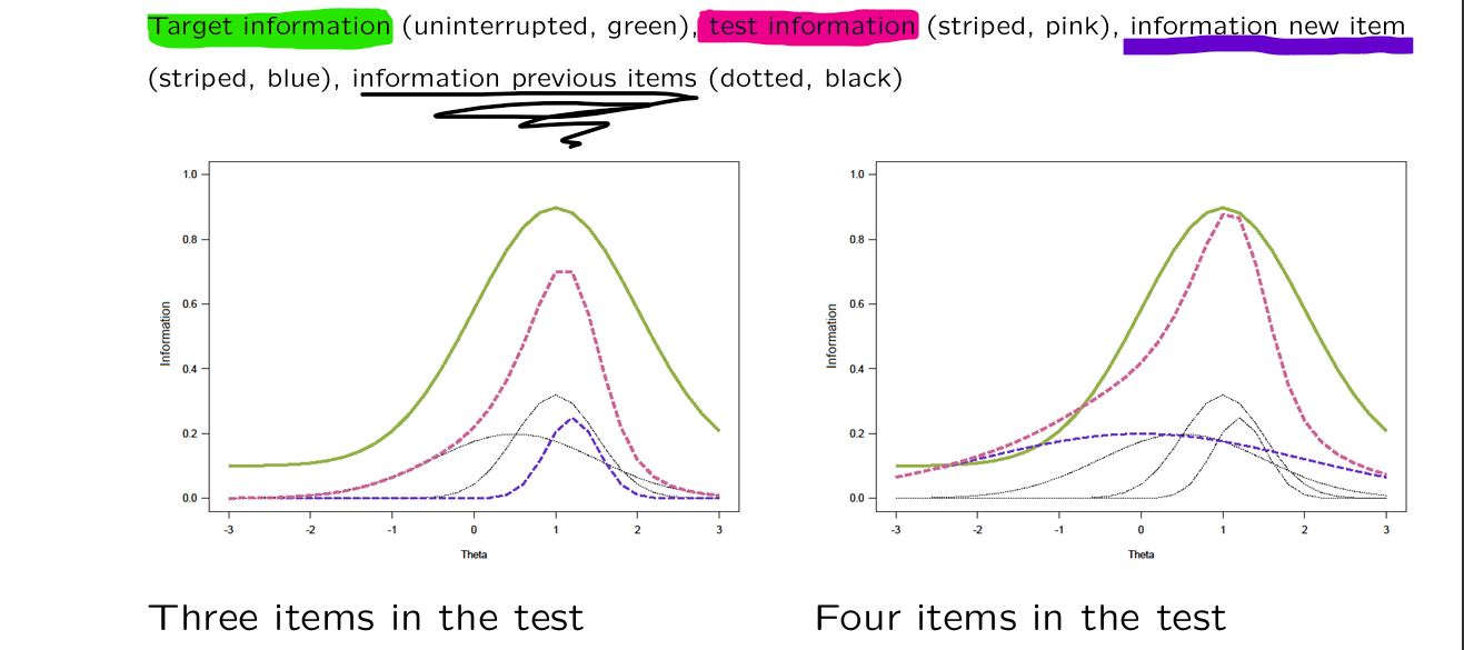
IRT allows for custom made tests
different purpose → different target information function → different test composition
this way we can develop tests that accurately measure in a specific population (high/low skilled group)
population-independent → results remain comparable
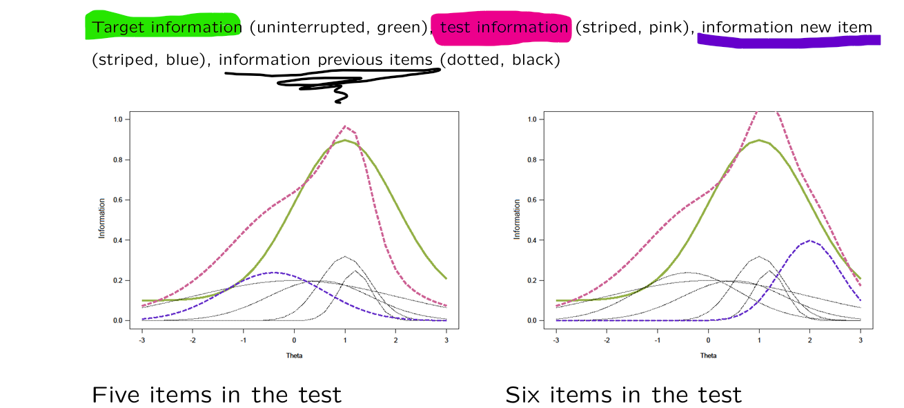
one step further: everyone gets a personalized test
Adaptive Tests
every respondent receives a unique custom-made test
items are selected so that their level matches the respondent’s ability
more efficient! we don’t waste the respondent’s time
item bank with items that satidfy