ELASTICITY AND REVENUE

Supply and Demand

Demand

• Relationship between demand and price

• What is the law of demand?

• As the price of a good or service decreases, the quantity demanded by consumers generally increases, and vice versa. This inverse relationship illustrates that consumers tend to buy more when prices are lower, adhering to the law of demand.

  • The law of demand.

  • The income effect.

  • The substitution effect.

• The demand curve:

  • The axes.

  • Individual and market demand curves.

Demand Curve Example: Potatoes (Monthly)

Market Demand Curve

The market demand curve is plotted with Price (pence per kg) on the Y-axis and Quantity (tonnes: 000s) on the X-axis.

• Point A: Price 20, Quantity 700

• Point B: Price 40, Quantity 500

• Point C: Price 60, Quantity 350

• Point D: Price 80, Quantity 200

• Point E: Price 100, Quantity 100

Movements Along and Shifts in the Demand Curve

• Change in price: Movement along the demand curve (change in quantity demanded).

• Change in any other determinant: Shift in the demand curve (change in demand).

  • Increase in demand: Rightward shift.

  • Decrease in demand: Leftward shift.

Increase in Demand

Possible causes:

• Tastes shift towards this product.

• Rise in price of substitute goods.

• Fall in price of complementary goods.

• Rise in income.

• Expectations of a rise in price.

Demand Functions

• Simple demand functions: $Qd = a – bP$

• Where:

• Qd = Quantity Demanded

• P = Price

Demand Curve Equation Example

• $Qd = 10000 – 200P$

• When P = 5, Qd = 9000

• When P = 10, Qd = 8000

• When P = 15, Qd = 7000

• When P = 20, Qd = 6000

Supply

• What is the law of supply? - PROFIT

• The law of supply states that, all else being equal, an increase in the price of a good or service will lead to an increase in the quantity supplied, and conversely, a decrease in price will result in a decrease in quantity supplied.

• The supply curve:

  • The axes.

  • Individual and market supply curves.

    Why do supply curves generally slope up?

  • The upward slope indicates that as prices rise, suppliers are willing to produce and sell more of a good or service in order to increase their profits.

Supply Curve Example: Potatoes (Monthly)

Market Supply Curve

The market supply curve is plotted with Price (pence per kg) on the Y-axis and Quantity (tonnes: 000s) on the X-axis.

• Point a: Price 20, Quantity 100

• Point b: Price 40, Quantity 200

• Point c: Price 60, Quantity 350

• Point d: Price 80, Quantity 530

• Point e: Price 100, Quantity 700

Other Determinants of Supply

• Costs of production

• Profitability of alternative products (substitutes in supply)

• Profitability of goods in joint supply

• Nature and other random shocks

• Aims of producers

• Expectations of producers

Movements Along and Shifts in the Supply Curve

• Change in price: Movement along the supply curve (change in quantity supplied).

• Change in any other determinant: Shift in the supply curve (change in supply).

  • Increase in supply: Rightward shift.

  • Decrease in supply: Leftward shift.

Supply Functions

• Simple supply function: $Qs = a + bP$

  • Where:

    • Qs = Quantity Supplied

    • P = Price

Price and Output Determination

• Equilibrium price and output

  • Response to shortages and surpluses

    • Shortage (D > S) => price rises

    • Surplus (S > D > price falls

  • Significance of ‘equilibrium’

Equilibrium Example: Potatoes (Monthly)

Market Equilibrium

The intersection of market demand and supply curves determines equilibrium.

Practice Example

The demand and supply functions for "AwesomeRay" are given by:

• Demand: $Qd = 1000 – 2P$

• Supply: $Qs = 200 + 2P$

Determine the output and price at equilibrium:

To find the equilibrium, set Qd equal to Qs:

$1000 - 2P = 200 + 2P$.

Solving for P, we get:

$1000 - 200 = 2P + 2P$

This simplifies to $800 = 4P$, hence $P = 200$.

Substituting P back into either the demand or supply function, we find the equilibrium quantity:

$Qd = 1000 - 2(200) = 600$.

Therefore, the equilibrium price is $200$ and the equilibrium quantity is $600$.

Effects of Shifts in the Demand Curve

• Movement along the supply curve and the new demand curve.

Effects of Shifts in the Supply Curve

• Movement along the demand curve and the new supply curve.

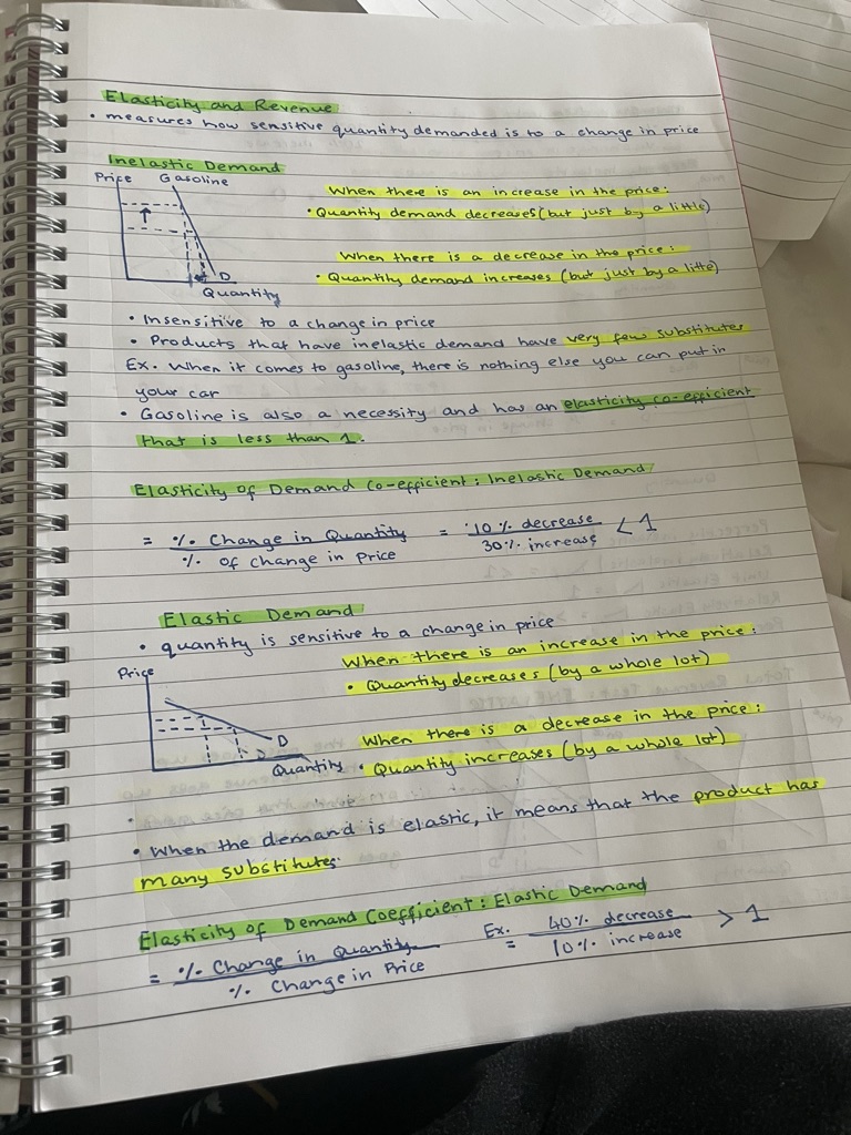
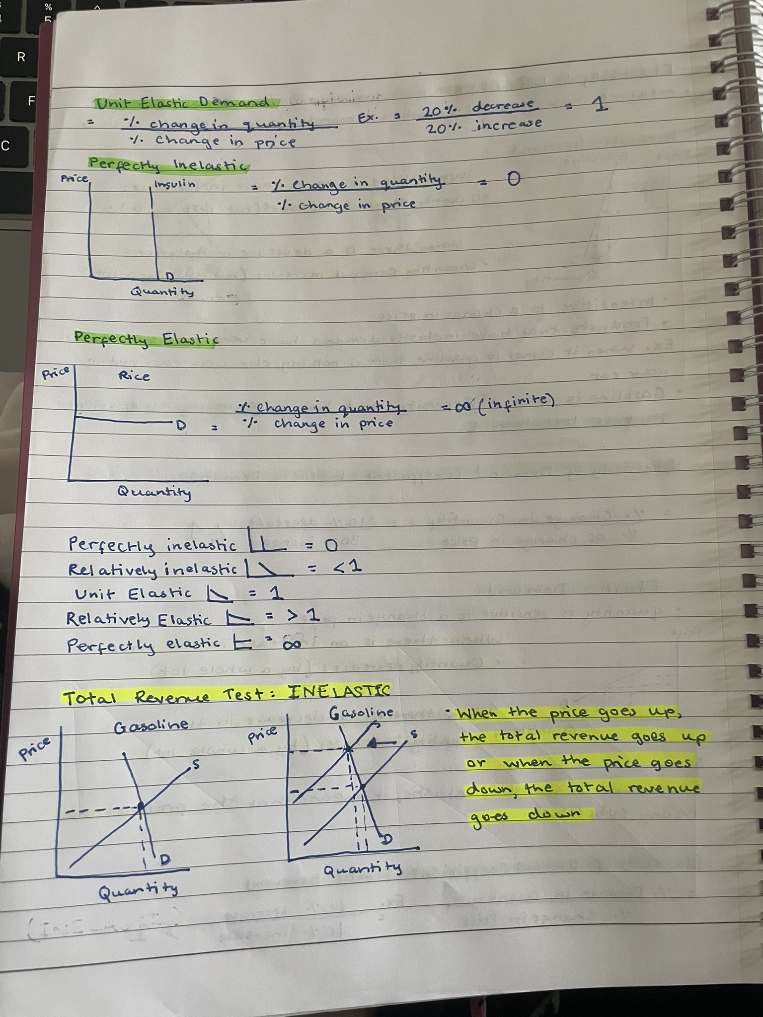
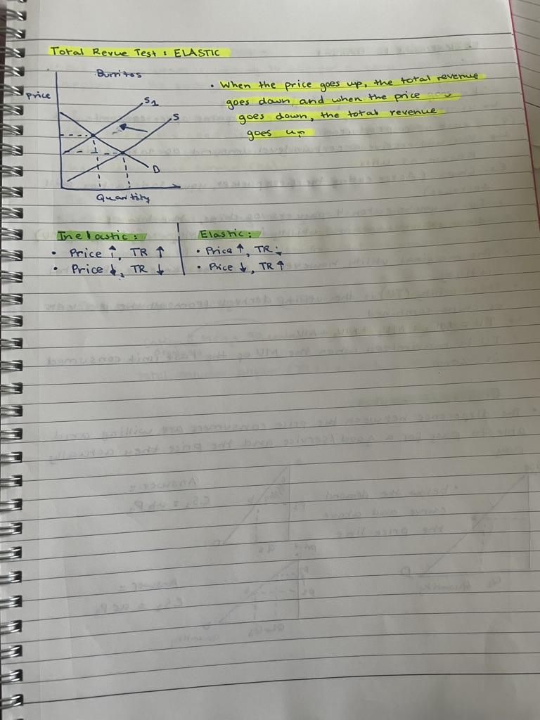
Elasticity and Revenue