Module 5: Labor and financial markets and elasticity

Labor market: the supply and demand for labor

• Law of demand in labor markets

  • Higher salary or wage (price) in the labor markets leads to a decrease in the quantity of labor demanded by employers

  • Lower salary or wage (price) leads to an increase in the quantity of labor demanded

  • Factors that can shift the demand curve for labor

    • demand for output

    • education and training

    • technology

    • number of companies (employers)

    • government regulations

    • price and availability of other inputs

• Law of supply in labor markets

  • Higher price for labor leads to higher quantity of labor supplied

  • lower price for labor leads to lower quantity supplied

  • factors that can shift the supply curve for labor

    • number of workers

    • education requirements

    • government policies

• equilibrium: the quantity supplied, and the quantity demanded are equal

  • at the equilibrium wage, employers can find workers and workers can find jobs

Technology and wages

• demand curve shifts

  • the graph shows that the demand curve for low level skills shifts to the left when technology can do the jobs previously done by workers

  • the right graph shows that the demand curve will shift to the right with increased use of technology in fields such as information technology and network administration

Price floors in the labor market

• salary or wage: money paid for work or for a service

• minimum wage: a price floor that makes it illegal for an employer to pay employees less than a certain hourly rate

• living wage: the amount a full-time worker would need to afford the essentials of life: food, clothing, shelter, and healthcare

Demand and supply in financial markets

• savings: supply of financial capital

• borrowing: demand for financial capital

• financial capital: economic resources measured in terms of money

• interest rate: the “price” of borrowing the financial market; a rate of return an Invesment

• usury laws: laws that impose an upper limit on the interest rate that lenders can charge

Demand and supply for borrowing money with credit cards

• In the above example of the market for credit cards borrowing, the demand (D) intersects with the supply curve (S) at an equilibrium (E) interest rate

• At equilibrium, the interest rate is 15% and the quantity of money demanded is $600 billion

• At a rate above equilibrium, more lenders would be willing to loan but less people would want to borrow (Surplus)

• At a rate below equilibrium, less lenders would be willing to take the risk and loan money, but more borrowers would want credit (Shortage)

Usury Laws (price ceiling)

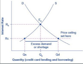
• in the above example, the original interest rate is R0 and the demand for borrowing is Q0

• Let’s assume that a law is passed banning high interest rates and sets the rate allowed below that shown above Rc

• In that case, you would have demand to borrow at the lower rate increase but have less suppliers at that rate (shortage)

The effect of growing U.S. debt

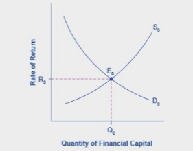
• the graph shows the demand for financial capital from and the supply of financial capital into the U.S. financial markets by foreign entities

• the equilibrium (E0) occurs at an equilibrium rate of return (R0) and at the equilibrium quantity (Q0) of financial capital

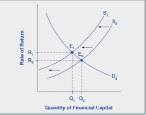
• The graph shows the interest of foreign entities to invest in the U.S> diminishes and the supply curve shifts to the left (S1)

• This would lead to a new equilibrium (E1), which occurs at the higher interest rate (R1), and the lower quantity of financial investment (Q1)

The Market systems as an efficient mechanism for information

• Demand and supply models:

  • Demand and supply curves explain existing levels of, and how economic events will cause changes in, prices and quantities

• The horizontal axis (“X” axis) shows the different measurements of quantity of:

  • a good or service

  • labor for a given job

  • financial capital

• The vertical axis (“Y” axis) shows a measure of price of:

  • a good or service

  • the wage in the labor market

  • the rate of return in the financial market

Effects of price controls on equilibrium prices and quantities

• changes in demand and supply reveal themselves through consumers’ and producers’ behavior

• price controls may deprive everyone in the economy of this critical information

• without his information, it becomes difficult for buyers and sellers to react as changes occur throughout the economy

Demand for nurses as baby boomers get older

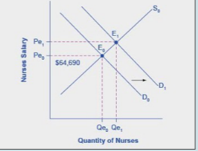
• in 2010, the median salary for nurses was $64,690

• as demand for nursing services increases, the demand curve shifts to the right from (D0 to D1) and the equilibrium quantity of nurses increases from Qe0 to Qe1

• the salary of nurses also increases from Pe0 to Pe1

impact of decreasing supply of nurses between 2014 and 2024

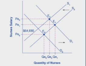
• but let’s suppose that the nursing population also gets older and many enter retirement

• this would cause a leftward shift of the supply curve which would result in higher salaries for the remaining nurses, at Pe2

• the higher salary could lead to more people choosing nursing as a profession or employers looking to find alternatives to nurses to lower their costs

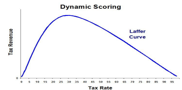
The Laffer Curve

The concept of elasticity of demand

• elasticity

  • is an economics concept that measures responsiveness of one variable to changes in another variable

• price elasticity of demand

  • the percentage change in the quantity of a good or service demanded divided by a change in price: (change in quantity demanded/ change in price)

• price of elasticity of supply

  • is the percentage change in the quantity supplied of a good or service divided by a change in price (change in quantity supplied/ change in price)

• elastic demand:

  • if the change in quantity demanded or supplied is greater than the increase in price — indicates a high responsiveness to price increases (%change in quantity> %change in price)

• inelastic demand

  • if the change in quantity demanded or supplied is less than the increase in price — indicates a low responsiveness to price increases (%change in quantity <%change in price)

• unitary demand

  • if the change in quantity demanded or supplied is equal to the increase in price — indicates a lack of responsiveness to price increases (%change in quantity = %change in price)