W4 L2 - Parametric statistics: assumptions (independence, homoscedasticity), Pearson correlation, and independent-samples t-tests
Homoscedasticity (equal variances)
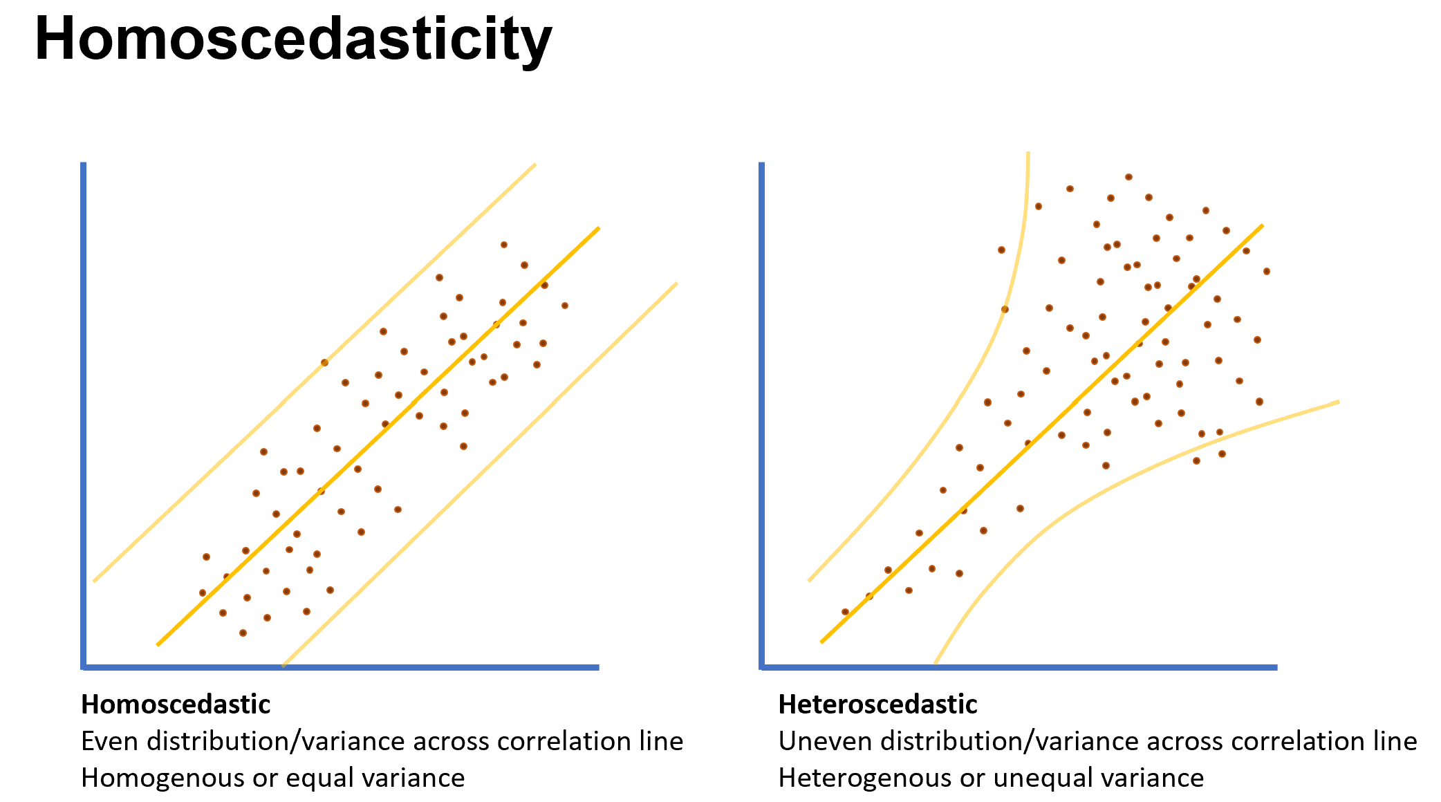
Definition: homoscedasticity = homogeneity of variance; an important assumption in parametric statistical models.
Visual assessment:
Left plot: data are homoscedastic (even variance across the correlation line).
Right plot: data are heteroskedastic (unequal variance across the correlation line; data fan out or cluster as you move along the axes).
Terminology:
Homoscedasticity = equality of variances across values of the predictor.
Heteroskedasticity = unequal variances.
Statistical testing:
Levene’s test is used to statistically test for homogeneity of variance.
Levene’s test provides a statistic F and a p-value:
Decision rule: if p < 0.05, then the assumption of equal variances is violated; if p \geq 0.05, the assumption is not violated.
Practical implications when violated:
For t-tests: use Welch’s t-test when variances are unequal.
For correlation: if obvious grouping/heterogeneity is present, consider a nonparametric alternative like Spearman’s correlation.
Practical note from practice:
Often data are explored visually for fan shapes or obvious data clumps indicating unequal variances.
Levene’s test provides a statistical check, complementing visual inspection.
Related tests mentioned:
Shapiro–Wilk test for normality (W statistic)
Levene’s test uses an F statistic, as above.
Independence
Definition: observations are independent (no two observations are related or affect each other).
Importance: independence is a core assumption for parametric tests; it is a logical/ design-based assumption, not something you test with a statistic like Levene’s or Shapiro–Wilk.
Examples illustrating violations:
Example 1 (non-independence): Gym participants sampled on Monday and Wednesday with 3 participants appearing in both days. This creates dependence between the two groups; to meet independence, those participants should be excluded.
Example 2 (non-independence): One instructor teaches two weight classes (old vs new method). If the same people could influence both groups, independence is violated.
Example 3 (independence): Each member is asked once about pool usage; this example is independent.
Takeaway: check study design for potential shared participants or cross-group influence; if independence is violated, adjust the analysis (e.g., exclude overlapping participants or model the dependence).
Pearson correlation (r) and its assumptions
What it measures:
Pearson correlation assesses a linear (straight-line) relationship between two variables.
Assumptions for Pearson correlation: 1) Linear relationship: the relationship should be approximately a straight line when plotting the data.
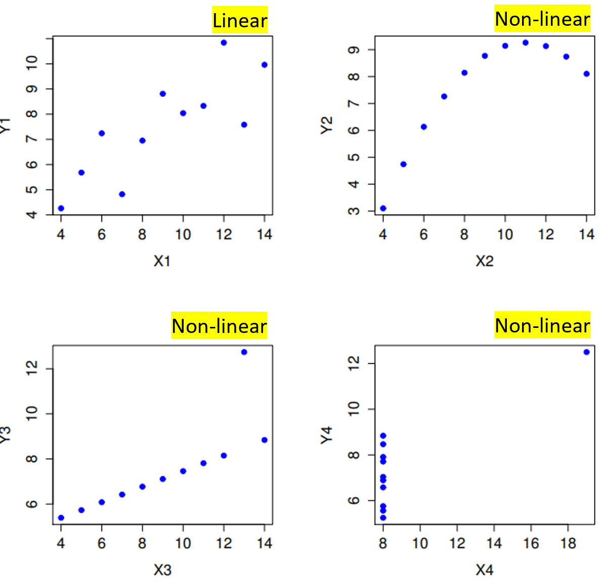
How to check: create a scatter plot; look for linearity. Nonlinear shapes (curve, U-shape, J-shape) indicate the relationship may not be well captured by a linear r.
2) Normality of the data (parametric): the data should be roughly normally distributed.
3) Homogeneity of variance (homoscedasticity) across the correlation line: variance should be similar at different levels of the predictor.
4) Independence: observations should be independent (see above).
5) Variable types: at least one variable should be continuous and the other should be continuous as well; dichotomous variables are not typical for Pearson correlation.
Practical note on dichotomous variables:
If one variable is dichotomous, a t-test is usually more appropriate when you want to compare group means (one group vs the other). Pearson correlation can technically be computed with one continuous and one dichotomous variable, but for interpretation in terms of group differences, a t-test is more efficient.
Range and interpretation of r:
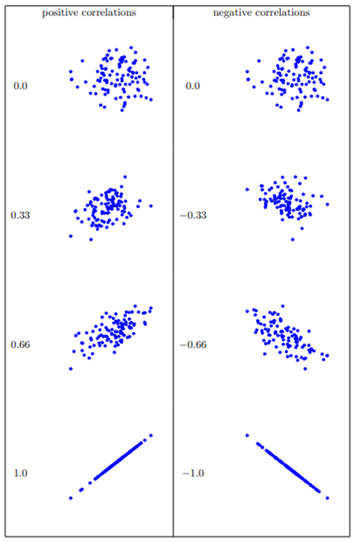
r varies between −1 and +1.
r = 0 indicates no linear relationship; r = +1 indicates a perfect positive linear relationship; r = −1 indicates a perfect negative linear relationship.
Negative values are indicated with a minus sign; positive values do not have a sign.
Example intuition: as you move through data, stronger linearity corresponds to higher |r| (closer to 1 or −1).
Misleading example (importance of visual inspection):
You can force the same r (e.g., r = 0.82) on several data patterns; but only some of those patterns are truly linear. Visual inspection shows that only some have a linear relationship; others are nonlinear despite having the same r value if forced.
r as a measure of effect size:
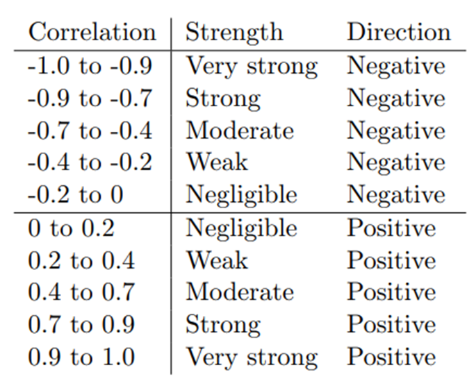
r is used as an effect size for the strength of the linear relationship.
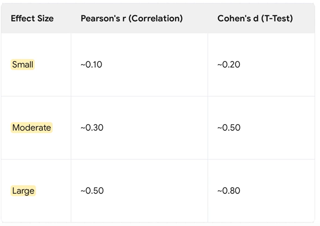
There are arbitrary cutoffs to interpret strength (small/medium/large), often taken from textbooks or APA guidelines; note that these cutoffs are conventional and not universally fixed.
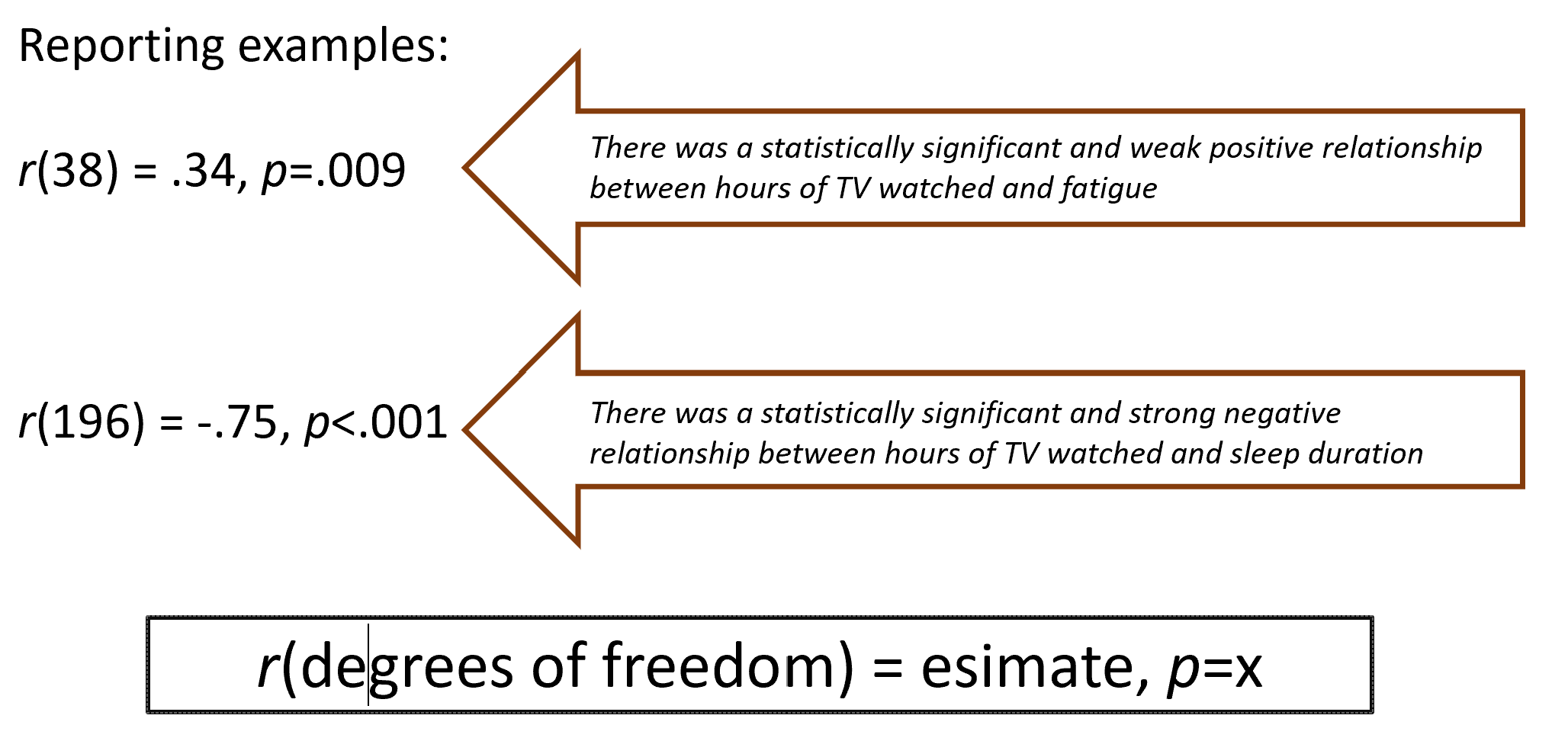
Reporting Pearson correlation (APA style examples):
Example 1:
r(38) = 0.34,\quad p = 0.009Interpretation: statistically significant and a weak-to-moderate positive relationship between the two variables (example: hours of TV watched and fatigue).
Example 2:
r(196) = -0.75,\quad p < 0.001Interpretation: statistically significant and a strong negative relationship (example: hours of TV watched and sleep duration).
Two different types of T-Tests
Independent: Two DIFFERENT groups (app users vs non users)
Paired: SAME group change over time (A persons age at Time 1 vs Time 2)
Between-subjects (independent samples) t-tests
Purpose:
Compare means between two groups on a continuous outcome when the grouping variable is dichotomous (two groups).
Assumptions for the dependent variable (outcome):
The dependent variable should be parametric (approximately normally distributed within groups).
The independent variable should be dichotomous (two groups).
Independence assumption (see above): observations between groups should be independent.
Homogeneity of variance (see above): variances of the dependent variable should be equal across groups.
Note on scope in the course:
The course focuses on between-groups (independent) t-tests; there are also within-subjects (paired) t-tests, which compare the same participants across two time points or conditions, but these are not the primary focus here.
Effect size for t-tests:
T-tests are not direct measures of effect size; Cohen’s d is used to quantify effect size.
Cohen’s d is computed from the t-test results and group means/variances (standardized mean difference).
Conventional cutoffs (from textbooks) are used to interpret small, medium, or large effects. Note these cutoffs are conventions and can vary by field.
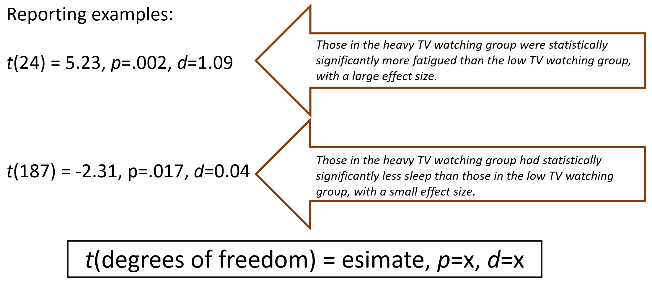
Reporting t-test results (APA style):
Report the t statistic, degrees of freedom, p-value, and Cohen’s d:
Example 1:
t(24) = 5.23,\quad p = 0.002,\quad d = 1.09Interpretation: those in the heavy TV-watching group were statistically more fatigued than those in the low TV-watching group, with a large effect.
Example 2:
t(187) = -2.31,\quad p = 0.017,\quad d = 0.04Interpretation: those in the heavy TV-watching group had statistically significantly less sleep than those in the low TV-watching group, with a small effect.
Practical notes for interpretation:
The sign of t indicates which group has the higher mean (positive t means group 1 > group 2 if group 1 is coded as the reference).
Always check descriptive statistics to determine which group is larger or higher before interpretation.
Use t-tests when your main question is about group differences.
Use correlation when your main question is about associations between variables.
Feature
T-test
Pearson Correlation
Goal
Compare means between groups
Measure relationship between variables
Variables
DV = continuous, IV = categorical (2 groups)
Both variables continuous
Example Question
Do men and women differ in exam scores?
Are study hours associated with exam scores?
Output
t-value, DF, p-value
r-value, DF, p-value
DF
One-sample: N−1, Two-group: N1+N2−2
N−2
Reporting and interpretation: general guidelines and practical tips
Always visualize data before applying stats (scatter plots for correlations; boxplots/histograms for t-tests).
Report all relevant statistics in APA style for clarity and reproducibility:
For correlation: r, df, p; example formats shown above.
For t-tests: t, df, p, and Cohen’s d; example formats shown above.
Be mindful of the direction of effects when interpreting signs of r or t and which group is considered reference.
Understand that some assumptions can be violated (e.g., non-normality, heteroscedasticity); there are robust alternatives (Spearman correlation, Welch’s t-test) and the choice should be guided by data inspection and the research question.
Quick practice checklist (from the transcript)
[ ] Check independence of observations (design-level check; avoid overlapping participants across groups).
[ ] Assess homoscedasticity (visual inspection of spread around the line; Levene’s test if formal check is desired).
[ ] Assess linearity for Pearson correlation (scatter plot; look for straight-line pattern).
[ ] Check normality of the dependent variable (Shapiro–Wilk test as a formal check).
[ ] Decide between Pearson r and Spearman if variance is not homogeneous or if relationships look non-linear.
[ ] Choose between independent-samples t-test or paired t-test based on study design (between-group vs within-subjects).
[ ] Report results with proper statistics: for correlation, r and p; for t-tests, t, df, p, and Cohen’s d.
[ ] Use descriptive statistics to determine which group is larger or has higher means before interpreting the sign in t-test results.
Connections to broader concepts
These topics connect to foundational principles of inferential statistics: sampling distribution, null hypothesis significance testing, and effect size interpretation.
The emphasis on assumptions (normality, linearity, homogeneity of variance, independence) mirrors standard practice across many parametric methods beyond correlation and t-tests.
The discussion of nonparametric alternatives (Spearman correlation) and robust tests (Welch’s t-test) highlights the practical flexibility needed when assumptions are violated in real data.
Summary of key formulas and symbols
Levene’s test (homogeneity of variance):
F = F{\text{Levene}}(df1, df2),\quad p = p{\text{Levene}}Shapiro–Wilk normality test:
W = W{\text{Shapiro}},\quad p = p{\text{Shapiro}}Pearson correlation (linear relationship between two continuous variables): r\in[-1, +1]
Example reporting: r(df) = 0.34,\quad p = 0.009 or r(df) = -0.75,\quad p < 0.001
Independent-samples t-test: t(df) = t{\text{value}},\quad p = p{\text{value}},\quad d = \text{Cohen's } d
Example 1: t(24) = 5.23,\quad p = 0.002,\quad d = 1.09
Example 2: t(187) = -2.31,\quad p = 0.017,\quad d = 0.04
Cohen’s d (effect size for t-tests): interpret via conventional small/medium/large cutoffs (context-dependent). (Cutoffs vary by source; common conventions include small ≈ 0.2, medium ≈ 0.5, large ≈ 0.8 in many fields.)