Comprehensive Guide to Integration Applications

Average Value of a Function

One of the most fundamental applications of the definite integral in AP Calculus AB is finding the average value of a continuous function over a specific interval. While an arithmetic mean sums discrete numbers and divides by the count, calculus allows us to average an infinite set of values along a curve.

Definition and Formula

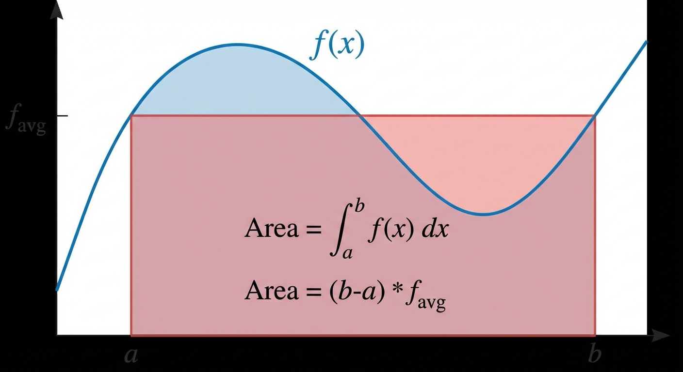
The average value of a continuous function $f(x)$ on the closed interval $[a, b]$ is defined as:

$f<em>{avg} = \frac{1}{b-a} \int</em>{a}^{b} f(x) \, dx$

Key Concept: Geometrically, $f{avg}$ is the height of a rectangle that has the same width $(b-a)$ and the same area as the region under the curve $f(x)$. This is related to the Mean Value Theorem for Integrals, which guarantees that a continuous function assumes its average value at least once in the interval (i.e., there exists a $c$ in $(a, b)$ such that $f(c) = f{avg}$).

Example 1

Find the average value of $f(x) = 3x^2$ on the interval $[0, 2]$.

Solution:

1. Identify $a=0$ and $b=2$. The width is $2-0 = 2$.
2. Set up the integral:
   $f<em>{avg} = \frac{1}{2} \int</em>{0}^{2} 3x^2 \, dx$
3. Integrate $3x^2$ to get $x^3$.
4. Evaluate:
   $f<em>{avg} = \frac{1}{2} [x^3]</em>{0}^{2} = \frac{1}{2} (2^3 - 0^3) = \frac{1}{2}(8) = 4$

The average value is 4.

Particle Motion (Rectilinear Motion)

In Unit 8, you apply integration to solve kinematic problems involving position, velocity, and acceleration of a particle moving along a line.

Relationships

Recall the derivative ladder: $s(t) \xrightarrow{d/dt} v(t) \xrightarrow{d/dt} a(t)$. Integration allows us to climb back up the ladder.

Net Change vs. Total Distance

This is the most critical distinction in this unit. Students often confuse displacement with distance traveled.

1. Displacement: The net change in position. This can be positive, negative, or zero.
   $\text{Displacement} = \int<em>{t</em>1}^{t<em>2} v(t) \, dt = s(t</em>2) - s(t_1)$

2. Total Distance Traveled: The sum of all movement, regardless of direction. We must integrate the absolute value of velocity (speed).
   $\text{Total Distance} = \int<em>{t</em>1}^{t_2} |v(t)| \, dt$

3. Current Position: To find the position at a specific time $t$, you generally need an initial condition (start position).
   $s(t) = s(0) + \int_{0}^{t} v(x) \, dx$
   "Current Position = Start Position + Displacement"

Common Pitfall: The Turning Point

When calculating Total Distance manually without a calculator, you must find where the particle turns around.

1. Set $v(t) = 0$ to find critical points.
2. Split the integral into intervals where $v(t)$ is positive and negative.
3. Integrate each piece and sum their absolute values.

Area Between Two Curves

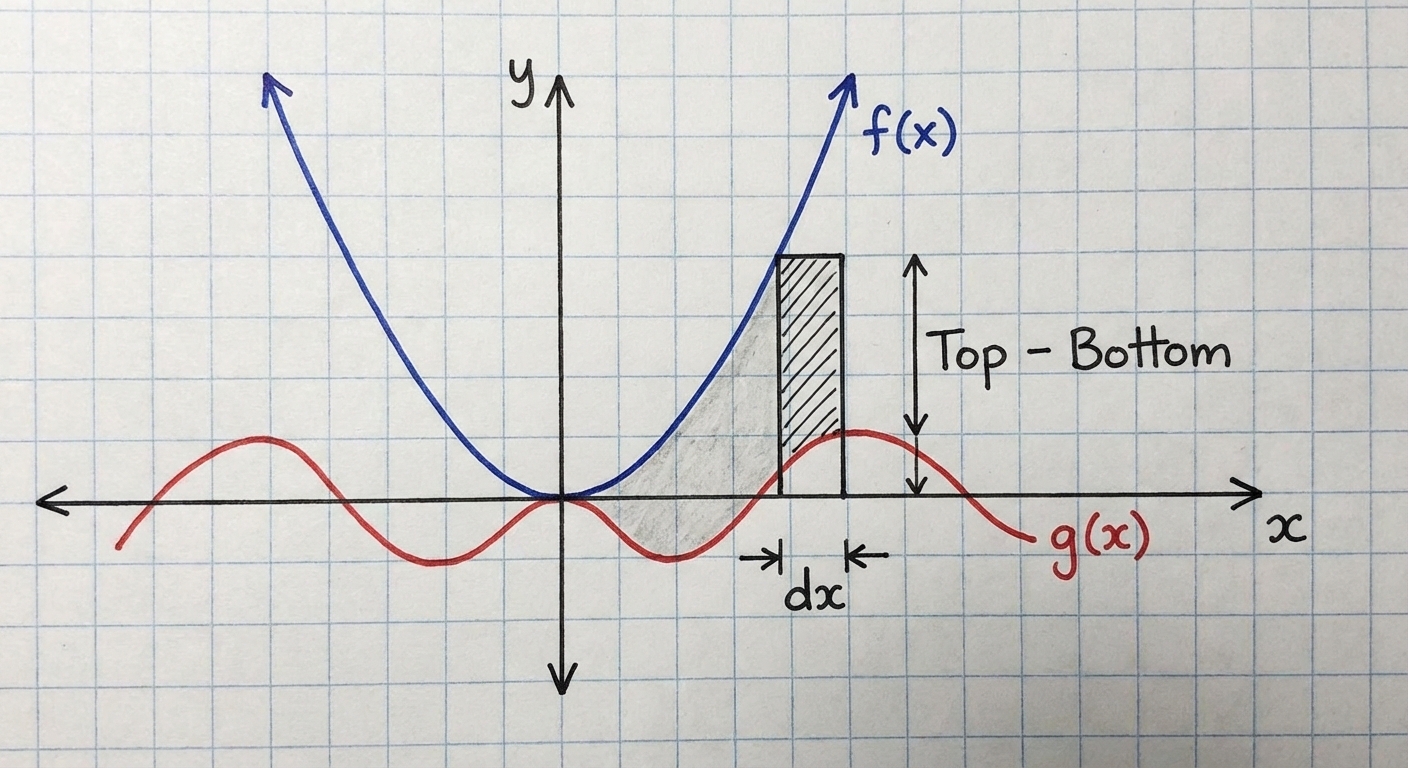
Previously, you found the area between a curve and the x-axis. Now, we calculate the area trapped between two functions, $f(x)$ and $g(x)$.

Vertical Slicing (Normally dx)

If the region is bounded by functions of $x$ (top and bottom), we use vertical representative rectangles.

$\text{Area} = \int_{a}^{b} [\text{Top}(x) - \text{Bottom}(x)] \, dx$

Steps:

1. Graph it (if allowed) to see which function is on top.
2. Find Intersections: Set $f(x) = g(x)$ to find the limits of integration $a$ and $b$, unless given.
3. Integrate the difference.

Horizontal Slicing (dy)

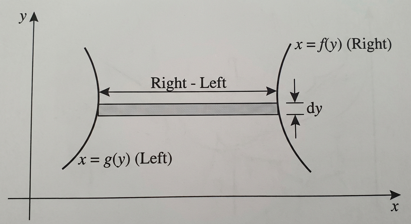
Sometimes curves are better defined as $x = f(y)$ (functions of $y$). In these cases, we slice horizontally.

$\text{Area} = \int_{c}^{d} [\text{Right}(y) - \text{Left}(y)] \, dy$

Note: All equations must be solved for $x$ in terms of $y$. The limits of integration ($c$ and $d$) correspond to y-values.

Example 2: Area Between Curves

Find the area bounded by $y = \sqrt{x}$ and $y = x^2$.

1. Intersection: $\sqrt{x} = x^2 \implies x = x^4 \implies x(x^3-1) = 0$. So, $x=0$ and $x=1$.
2. Top vs Bottom: On $(0, 1)$, $\sqrt{x}$ is above $x^2$ (e.g., test $x=0.25$, $\sqrt{0.25}=0.5$, $0.25^2=0.0625$).
3. Setup: $\int<em>{0}^{1} (\sqrt{x} - x^2) \, dx = \int</em>{0}^{1} (x^{1/2} - x^2) \, dx$.
4. Solve: $[\frac{2}{3}x^{3/2} - \frac{1}{3}x^3]_0^1 = (\frac{2}{3} - \frac{1}{3}) - 0 = \frac{1}{3}$.

Volumes with Known Cross-Sections

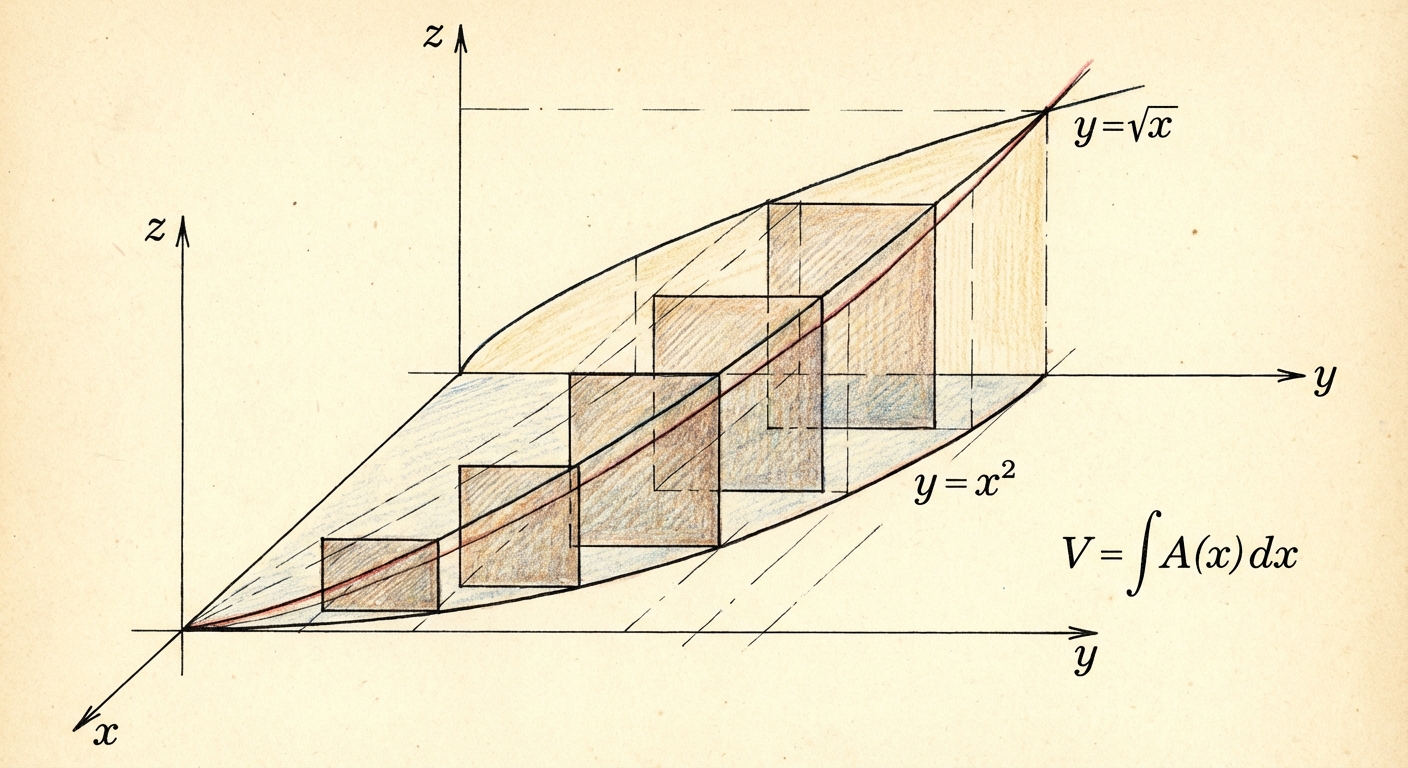
In these problems, a 2D base region is defined by functions in the xy-plane, and 3D shapes pop out of the page perpendicular to this base.

General Concept

Volume is the accumulation of area slices.
$V = \int_{a}^{b} A(x) \, dx$
where $A(x)$ is the area formula for the specific geometric shape of the cross-section.

Common Cross-Section Formulas

Let $s = \text{Top} - \text{Bottom}$ (the length of the slice in the base).

Note on Semicircles: The diameter is $s$, so radius $r = s/2$. Area is $\frac{1}{2}\pi (s/2)^2 = \frac{\pi}{8}s^2$.

Volumes of Revolution

These are 3D solids created by spinning a 2D area around an axis (like the x-axis, y-axis, or another line).

1. The Disk Method (No Holes)

Used when the region being rotated touches the axis of rotation completely (no gaps).

$V = \pi \int_{a}^{b} [R(x)]^2 \, dx$

• $R(x)$: The radius, measured from the axis of rotation to the outer edge of the function.

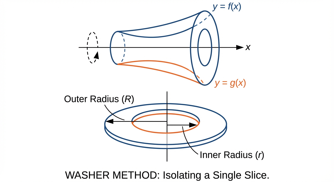
2. The Washer Method (Holes)

Used when there is a gap between the region and the axis of rotation. The resulting 3D cross-section looks like a washer (a donut).

$V = \pi \int_{a}^{b} ([R(x)]^2 - [r(x)]^2) \, dx$

• $R(x)$ (Outer Radius): Distance from axis of rotation to the far curve.
• $r(x)$ (Inner Radius): Distance from axis of rotation to the near curve.

Important Rules for Axes of Rotation

• Revolving around x-axis: Use $dx$. ($y=…$)
• Revolving around y-axis: Use $dy$. ($x=…$)
• Revolving around $y = k$: Radii are vertical distances. $R(x) = |\text{Top} - k|$.
• Revolving around $x = h$: Radii are horizontal distances. $R(y) = |\text{Right} - h|$.

Common Mistakes & Pitfalls

1. Displacement vs. Distance:

   • Mistake: Calculating $\int v(t) dt$ when asked for Total Distance.
   • Correction: Always use $\int |v(t)| dt$ for total distance. If you don't have a calculator, split the integral at zeroes.

2. Square of the Difference vs. Difference of Squares:

   • Mistake: In the Washer Method, writing $\pi \int (R - r)^2 dx$.
   • Correction: It is mathematically $\text{Volume}<em>{\text{outer}} - \text{Volume}</em>{\text{inner}}$, so it must be $\pi \int (R^2 - r^2) dx$.

3. Forgetting $\pi$:

   • Mistake: Omitting the $\pi$ coefficient in Disk/Washer problems.
   • Correction: Remember, you are summing circle areas ($A=\pi r^2$). The $\pi$ is mandatory.

4. Initial Position:

   • Mistake: Thinking $\int_0^t v(t) dt$ is the position.
   • Correction: That is only the change in position. You must add the starting position $s(0)$.

5. Limits of Integration:

   • Mistake: Using x-values for limits when integrating with respect to $y$ (dy).
   • Correction: If the differential is $dy$, the limits must be $y$-values $(y1$ to $y2)$.