MRI Notes
MRI physics overview | MRI Physics Course | Radiology Physics Course #1
Here is a brief summary of the main points covered in the video "MRI physics overview":
MRI imaging uses signals from within the patient to generate images.
The Cartesian plane is used to localize the signal source.
Nuclear magnetic resonance is used to induce resonance in hydrogen atoms within the patient.
Hydrogen atoms act like tiny bar magnets with a magnetic moment.
A large magnetic field causes hydrogen atoms to align with the field and precess around their own axis.
The precessional frequency of hydrogen atoms is determined by the strength of the magnetic field.
Net magnetization vector, which is the combination of all magnetic moments, is aligned along the longitudinal axis.
A radio frequency (RF) pulse is used to move the net magnetization vector perpendicular to the main magnetic field, allowing for measurement.
The RF pulse must match the precessional frequency of the hydrogen atoms.
Flip angle is the angle at which the net magnetization vector is flipped by the RF pulse.
The movement of the net magnetization vector in the transverse plane induces a current in a receiver coil, which is used to generate the image.
When the RF pulse is stopped, the protons go out of phase, resulting in a decrease in transverse magnetization and signal. This decay is represented by the free induction decay (FID) curve or T2 curve*.
Different tissues have different T2* curves.
Longitudinal magnetization is regained as the net magnetization vector returns to alignment with the main magnetic field. This recovery is known as T1 recovery.
T1 recovery and T2 decay happen independently of each other.*
Time of echo (TE) is the time from the RF pulse to the measurement of the signal.
Time of repetition (TR) is the time from one RF pulse to the next.
Manipulating TE and TR times allows for the generation of different image contrasts.
Short TR times emphasize differences in T1 recovery, creating a T1 image.
Long TR times emphasize differences in T2 decay, creating a T2 image.
Different pulse sequences are used to generate images.
K space is used to encode the different slices on an MRI image.
MRI Machine - Main, Gradient and RF Coils/ Magnets | MRI Physics Course | Radiology Physics Course #2
Here is a summary of the main points from the video "MRI Machine - Main, Gradient and RF Coils/Magnets":
The MRI machine uses multiple magnets to create the magnetic fields needed for imaging.
Main Coil:
The outermost layer of the MRI machine.
Generates the B0 or main magnetic field, which runs along the longitudinal (Z) axis.
The strength of the main magnetic field depends on:
The number of coils of wire.
The amount of current running through the wire.
Uses a superconductor (typically niobium-titanium alloy) to generate sufficient current without resistance.
Requires liquid helium to maintain the superconductor at a temperature below 4 degrees Kelvin.
Quenching: A safety feature that releases helium gas if superconductivity is lost.
Shims:
Structures within the main coil that manipulate the main magnetic field to make it more homogeneous.
Passive shims: Magnetic sheets or ferromagnetic metal placed within the bore of the machine.
Active shims: Coils with their own electricity supply that can be adjusted to alter the magnetic field.
Can be superconductive (within the helium) or resistive (within the bore).
Gradient Coils:
The next layer of the MRI machine, lying perpendicular to each other in the X, Y, and Z planes.
Apply a gradient along the main magnetic field, changing its strength along different axes.
Do not change the direction of the main magnetic field.
By altering the magnetic field strength, they change the precessional frequency of hydrogen protons along the axes.
This is the foundation for spatial encoding of the MRI signal.
Isocenter: The part of the magnetic field that remains unchanged by the gradient coils.
Radio Frequency (RF) Coil:
Generates a magnetic field perpendicular to the main magnetic field (in the transverse or XY plane).
Emits an alternating magnetic field (RF pulse) that matches the precessional frequency of specific hydrogen protons.
This causes the targeted hydrogen protons to:
Fan out, increasing their angle from the main magnetic field (flip angle).
Become in phase with each other.
Allows for the selection of specific slices (slice selection) and the measurement of signal in the transverse plane.
Spin, Precession, Resonance and Flip Angle | MRI Physics Course | Radiology Physics Course #3
Here is a summary of the main points from the video "Spin, Precession, Resonance, and Flip Angle":
Nuclear magnetic resonance (NMR) governs how certain nuclei respond to external magnetic fields in MRI.
Spin:
Classical Model:
Describes a charged particle rotating on its axis, inducing a magnetic field.
This magnetic field is represented by the magnetic moment (a vector).
This model is not entirely accurate, as it cannot explain certain phenomena like the magnetic moment of a neutron.
Quantum Mechanical Model:
Spin is a fundamental quantum property of particles, like charge or mass.
It describes how a particle will react to an external magnetic field, referred to as spin angular momentum.
Protons, neutrons, and electrons have a spin value of ½.
Nuclei with an even number of protons and neutrons have a net spin of zero and are not affected by external magnetic fields.
Hydrogen, with one proton, has a non-zero spin and is therefore used in MRI.
Hydrogen in MRI:
Hydrogen is the most abundant element in the body and has the largest magnetic moment among NMR-active isotopes, making it ideal for MRI.
Free hydrogens, protons, and spins are used interchangeably to refer to hydrogen in MRI.
Gyromagnetic Ratio:
Links the magnitude of the magnetic moment to the spin of a particle.
The gyromagnetic ratio for hydrogen is 42.5 megahertz per Tesla.
Multiplying the gyromagnetic ratio by the magnetic field strength gives the Larmor frequency.
Larmor Frequency:
The precessional frequency of an atom in a magnetic field.
Determined by the gyromagnetic ratio of the atom and the strength of the magnetic field.
Used to calculate the frequency of the RF pulse needed to induce resonance.
Precession:
When placed in a magnetic field, hydrogen atoms align with the field and precess around their axis at the Larmor frequency.
The net magnetization vector, representing the sum of all magnetic moments, lies along the longitudinal (Z) axis.
Although individual hydrogen atoms are precessing, the net magnetization vector does not precess because the transverse magnetization values cancel each other out.
Resonance:
Occurs when an RF pulse with a frequency matching the Larmor frequency is applied.
Causes two things to happen:
The net magnetization vector is tipped away from the longitudinal axis, gaining transverse magnetization.
The precessing hydrogen spins become in phase with each other.
Resonance allows for the measurement of signal and the selection of specific slices.
Flip Angle:
The angle at which the net magnetization vector is tipped away from the longitudinal axis by the RF pulse.
The larger the flip angle, the greater the transverse magnetization and signal strength.
A 90-degree flip angle yields the maximum signal.
Transverse Magnetization:
Only present when hydrogen nuclei are in phase (resonating).
It takes time for transverse magnetization to build after applying the RF pulse.
Short flip angles can be used to measure signal more quickly while still generating a significant signal.
180-Degree Flip Angle:
Possible due to the quantum properties of protons, even though the classical model would suggest otherwise.
Flips the net magnetization vector to a higher energy state, anti-parallel to the main magnetic field.
Used in certain pulse sequences to generate a true T2 signal.
T2 Relaxation, Spin-spin Relaxation, Free Induction Decay, Transverse Decay | MRI Physics Course #4
T2 Relaxation Terminology
Spin-spin Relaxation: The primary mechanism behind T2 relaxation is the interaction between spins. As the RF pulse is turned off, spins that were precessing in phase begin to dephase, causing a decrease in the net transverse magnetization. This dephasing is primarily due to spins transferring energy between each other.
Transverse Decay: As protons dephase, they lose their transverse magnetization, resulting in signal loss. This is also referred to as T2 decay.
T2 Relaxation Explained
After a 90-degree RF pulse, the net magnetization vector lies entirely in the transverse plane.
When the RF pulse is switched off, spins begin to dephase as they interact with each other. This occurs at different rates depending on the tissue.
Fat, with its long triglyceride chains, experiences more spin-spin interactions and faster T2 decay compared to water (CSF), where molecules can move more freely.
The T2 relaxation curve represents the decay of the transverse magnetization signal over time.
T2 vs. T2*
T2 Decay:* The actual measured decay of the transverse magnetization signal.
T2 Decay: Represents the loss of transverse magnetization due solely to spin-spin interactions (an ideal scenario).
T2 decay is always faster than T2 decay* because it's influenced by magnetic field inhomogeneities.
The T2 time constant* is the time it takes for 63% of the transverse signal to be lost.
Magnetic Field Inhomogeneities
Contribute to the difference between T2 and T2*.
Causes:
Imperfect magnetic field generation by the MRI scanner itself
Substances within the patient that disrupt local magnetic fields (e.g., metal, calcium)
Dephasing spins disrupting the local magnetic field
Inhomogeneous magnetic fields mean that protons in different locations experience different field strengths, causing them to precess at different rates, leading to faster dephasing and a more rapid loss of transverse magnetization (T2* decay).
Compensating for T2* Decay: Spin Echo
A 180-degree RF pulse can be applied to rephase spins that have dephased due to magnetic field inhomogeneities.
This pulse flips the spins 180 degrees, effectively reversing their dephasing trajectory.
By waiting the same amount of time after the 180-degree pulse as between the 90-degree and 180-degree pulses, the spins will rephase, resulting in an echo of the original signal.
This echo represents the T2 relaxation, as it accounts for the dephasing caused by magnetic field inhomogeneities.
Time of Echo (TE) and T2 Contrast
TE: The time between the initial 90-degree RF pulse and the measurement of the echo.
TE can be manipulated to highlight T2 differences between tissues.
Short TE: High signal, little T2 contrast
Longer TE: Lower signal, increased T2 contrast (tissues with longer T2 times will appear brighter)
Very Long TE: Very low signal, minimal contrast
The video concludes by stating that the next discussion will cover T1 relaxation and how it can be used to create T1 contrast in images.
Rephasing Clarification
Q: Don't the lectures suggest that TE is taken at the point when the spins rephase and create the strongest signal, which is when you can’t differentiate the signals from different tissues, or am I misunderstanding?
TLDR: We take a range of measurements around the peak signal.
A: You've hit on a point that often causes confusion! The lectures may give the impression that the TE measurement coincides with the peak signal from re phased spins, but this isn't entirely accurate. It's easy to misinterpret this, especially when initially learning about T2 relaxation and spin echoes.
Let's revisit why the TE is actually measured after the point of maximum rephasing:
Highlighting T2 Differences is the Goal: The purpose of a T2-weighted image is to demonstrate the variations in T2 decay rates between different tissues. If we measured the signal at the moment of perfect rephasing (TE/2), all tissues would exhibit the same strong signal, and the contrast based on T2 relaxation would be lost.
Contrast Arises from Decay After Rephasing: While the 180-degree RF pulse rephases spins and creates a peak signal, it's crucial to remember that T2 decay continues to occur even after this rephasing. Tissues with longer T2 times will lose signal more slowly than those with shorter T2 times.
TE Timing Captures Decay Differences: By strategically delaying the TE measurement to a point after the peak signal, we allow enough time for the T2 decay differences to become noticeable. This difference in signal strength at the TE is what generates the contrast in a T2-weighted image.
Consider these points from the sources that support this understanding:
Sampling at Multiple Points Surrounding TE: Source states, "...instead of sampling at one point at te we sample at multiple points surrounding te..." This suggests that data points are acquired over a range, capturing the changes in signal intensity as the spins dephase.
Signal Intensity Changes Over Time Surrounding TE: Source emphasizes, "...we want to remember that this signal intensity changes over time surrounding that te..." This reinforces the idea that the signal is not static at the TE but evolves as T2 decay progresses.
To clarify the relationship between spin rephasing and TE:
90-degree RF pulse: Tips the net magnetization vector into the transverse plane, creating maximum signal.
Dephasing: Spins begin to dephase due to T2 and T2* effects, leading to signal loss.
180-degree RF pulse: Refocuses the spins, reversing the dephasing order.
Peak Signal at TE/2: Spins are perfectly re phased at the midpoint between the 90-degree pulse and the TE, generating the strongest signal.
Continued Decay: T2 decay continues, with different tissues losing signal at different rates.
TE Measurement: The signal is measured at a time point after TE/2, allowing enough time for T2 contrast to develop.
In essence, while the strongest signal occurs at TE/2 due to spin rephasing, the TE measurement is intentionally delayed to a later time point to emphasize the differences in T2 decay rates and create a T2-weighted image.
T1 Relaxation, Spin-lattice Relaxation, Longitudinal Recovery | MRI Physics Course #5
What is T1 Relaxation?
T1 relaxation, also called spin-lattice relaxation or longitudinal recovery, involves spins interacting with the "lattice". The lattice refers to the non-spinning structural components of tissues, such as macromolecules and proteins.
This interaction causes the spins to realign with the main magnetic field (B0), leading to an increase in the net longitudinal magnetization vector.
T1 Relaxation vs. T2 Relaxation
T1 relaxation (longitudinal recovery) involves gaining longitudinal magnetization.
T2 relaxation (transverse decay) involves losing transverse magnetization. The previous summary of the video "T2 Relaxation..." covered the mechanisms of T2 relaxation in detail.
How T1 Relaxation Works
After a 90-degree RF pulse, the net magnetization vector is flipped into the transverse plane, and longitudinal magnetization is zero.
When the RF pulse is turned off, the spins begin to interact with the lattice, releasing energy and gradually realigning with the B0 field.
Different tissues have different T1 relaxation rates.
CSF, with fewer macromolecules, has a slower T1 relaxation rate because there are fewer interactions with the lattice to promote realignment.
Fat, with its long triglyceride chains and more structural components, has a faster T1 relaxation rate. The movement of these chains further enhances interactions with the lattice, leading to faster longitudinal recovery.
Visualizing T1 Relaxation
Imagine a room full of people spinning basketballs on their fingers (representing spins).
Obstacles in the room, like chairs (representing the lattice), cause the people to trip and the basketballs to tip, aligning with the direction of gravity (representing the B0 field).
In CSF, there are fewer "obstacles", so the spins take longer to realign.
In fat, there are more "obstacles", causing spins to realign more quickly.
T1 Time Constant
The T1 time constant is the time it takes for a tissue to regain 63% of its longitudinal magnetization.
T1 time constants are longer for CSF than for fat.
Why No T1*?
Unlike T2 relaxation, T1 relaxation is not significantly affected by magnetic field inhomogeneities.
While inhomogeneities cause some spins to regain longitudinal magnetization faster or slower, the overall effect averages out. The T1 time constant reflects this average rate of longitudinal recovery.
Highlighting T1 Differences: TR (Time to Repetition)
Since we can't directly measure longitudinal magnetization, we use TR (time to repetition) to highlight T1 differences in images.
A 90-degree RF pulse flips the net magnetization vector into the transverse plane.
The signal is sampled after a time TE (time to echo), which reflects T2 differences.
After a period TR, the 90-degree RF pulse is repeated. This is the "repetition" part of TR.
The amount of longitudinal magnetization regained during TR determines the strength of the signal when the next RF pulse is applied.
Short TR: Tissues with faster T1 recovery (like fat) will have regained more longitudinal magnetization and produce a stronger signal. This creates T1-weighted images, where fat appears bright and CSF appears dark.
Long TR: All tissues have time to fully recover their longitudinal magnetization, minimizing T1 differences.
Image Weighting
Manipulating TE and TR allows us to create images with different weightings:
T1-weighted: Short TR, short TE (emphasizes T1 differences).
T2-weighted: Long TR, long TE (emphasizes T2 differences).
Proton Density-weighted: Long TR, short TE (minimizes both T1 and T2 differences, primarily reflects the density of protons).
Why does only some magnetization recover when TR is short
TLDR: Only the vectors that have completely realigned with the longitudinal plane will be flipped. Since tissues with a shorter T_1 will have more realigned in the longitudinal plane, then more will be flipped to the transverse plane.
When using a short TR (time to repetition), not all longitudinal magnetization is recovered before the next RF pulse is applied. This means that different tissues, which have varying T1 recovery rates, will have different amounts of longitudinal magnetization available to be flipped into the transverse plane by the next RF pulse. Tissues with shorter T1 times, like fat, will have recovered more of their longitudinal magnetization and therefore produce a stronger transverse magnetization signal after the RF pulse. Conversely, tissues with longer T1 times, like CSF, will have recovered less longitudinal magnetization, resulting in a weaker transverse magnetization signal. Therefore, a short TR highlights T1 differences between tissues by capitalizing on the varying degrees of longitudinal magnetization recovery and their subsequent conversion into transverse magnetization.
T1, T2 and Proton Density Weighting | MRI Weighting and Contrast | MRI Physics Course #6
Review of T1 and T2 Relaxation
T2 Relaxation (Transverse Decay): The process of losing transverse magnetization due to spins dephasing. The T2 constant is the time it takes for a tissue to lose 63% of its transverse magnetization.
T1 Relaxation (Longitudinal Recovery): The process of regaining longitudinal magnetization as spins realign with the B0 field. The T1 constant is the time it takes for a tissue to regain 63% of its longitudinal magnetization.
Important Points About Relaxation
T2 relaxation occurs much faster than T1 relaxation. The loss of transverse magnetization happens rapidly as spins dephase, while regaining longitudinal magnetization is a slower process.
The initial strength of the longitudinal magnetization vector (before the 90-degree RF pulse) determines the strength of the transverse magnetization vector (after the 90-degree RF pulse). This means that tissues with a higher density of free hydrogen protons will have a stronger initial longitudinal magnetization and a stronger transverse magnetization after the RF pulse.
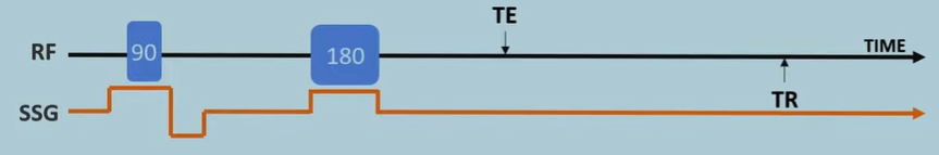
The Basic Pulse Sequence
A 90-degree RF pulse flips the net magnetization vector into the transverse plane.
TE (Time of Echo): The time after the RF pulse when the transverse magnetization signal is measured. Changing TE affects T2 contrast.
TR (Time of Repetition): The time between successive 90-degree RF pulses. Changing TR affects T1 contrast.
Manipulating TE for T2 Contrast
Short TE: All tissues have high signal with little contrast because there hasn't been enough time for significant T2 decay (dephasing) to occur.
Medium TE: Signal decreases, but T2 contrast increases. Tissues with longer T2 times (like CSF) will have higher signal than tissues with shorter T2 times (like muscle).
Long TE: Signal is very low, and contrast is minimal.
Manipulating TR for T1 Contrast
Short TR: Tissues with faster T1 recovery (like fat) will have regained more of their longitudinal magnetization before the next RF pulse. This creates T1-weighted images where fat appears bright.
Long TR: All tissues have enough time to fully recover their longitudinal magnetization, minimizing T1 differences and reducing contrast.
Image Weighting: Combining TE and TR
By adjusting TE and TR, we can create images that emphasize different tissue characteristics:
T1-weighted image: Short TR, short TE. Highlights T1 differences, showing tissues with faster T1 recovery (like fat) as bright.
T2-weighted image: Long TR, long TE. Highlights T2 differences, showing tissues with longer T2 times (like CSF) as bright.
Proton density-weighted image: Long TR, short TE. Minimizes both T1 and T2 differences, so the image primarily reflects the density of protons in each tissue.
Important Notes on Image Weighting
The absolute number of protons in a tissue also affects signal intensity. Tissues with more free hydrogen protons will have higher signal regardless of weighting.
Remember that every image has some contribution from both T1 and T2 relaxation. Weighting just emphasizes one type of contrast over the other.
The video concludes by providing typical ranges for TE and TR values used for different weightings:
Long TR: 2000 milliseconds (or in the high hundreds to 2000 range).
Short TR: 300-600 milliseconds.
Long TE: 80-160 milliseconds.
Short TE: 10-30 milliseconds.
Knowing these general ranges can help you determine the type of weighting used in an image based on the TE and TR values provided.
MRI Slice Selection | Signal Localisation | MRI Physics Course #7
The video "MRI Slice Selection | Signal Localisation" delves into the critical process of spatial localization in MRI, explaining how the machine determines the precise origin of signals within the patient's body. This detailed summary breaks down the key concepts presented:
The Need for Spatial Localization
Unlike imaging techniques like X-rays, where signals originate from an external source, the signals in MRI come from the patient themselves.
Therefore, we need a method to pinpoint the exact location of these signals within the three-dimensional space of the patient's body. This is achieved through spatial localization.
Spatial Localization in MRI
Spatial localization uses the Cartesian coordinate system (X, Y, and Z axes) to define the position of signals.
Z-axis (longitudinal axis): Runs from head to toe.
X and Y axes: Define the transverse (axial) plane.
The video focuses on slice selection, the process of isolating signals along the Z-axis. Subsequent videos will cover localization along the X and Y axes.
Slice Selection: The Basics
MRI images are composed of individual slices stacked together, each with a certain thickness.
Slice selection uses a slice selection gradient (a magnetic field gradient applied along the Z-axis) to differentiate the resonance frequencies of protons at different positions along this axis.
How Slice Selection Works
Applying the Slice Selection Gradient: A magnetic field gradient is applied along the Z-axis, resulting in varying magnetic field strengths at different points along the patient's length.
Different Resonance Frequencies: Due to the gradient, protons at different positions along the Z-axis experience different magnetic field strengths and, consequently, precess at different Larmor frequencies. (Recall the Larmor equation: Larmor frequency = gyromagnetic ratio * magnetic field strength).
Selective Excitation with an RF Pulse: An RF pulse with a specific bandwidth (a range of frequencies) is applied. Only protons precessing at frequencies within this bandwidth will undergo resonance and be flipped into the transverse plane.
Isolating the Slice: By carefully tuning the RF pulse frequency and bandwidth, we can selectively excite protons within a specific slice along the Z-axis, effectively isolating signals from that region.
Manipulating Slice Position and Thickness
Moving the Slice: The selected slice can be moved along the Z-axis by:
Changing the RF pulse frequency to target a different Larmor frequency.
Adjusting the slice selection gradient strength.
Physically moving the patient within the MRI machine.
Changing Slice Thickness: The thickness of the selected slice can be adjusted by:
Changing the bandwidth of the RF pulse: A wider bandwidth excites a thicker slice.
Changing the steepness of the slice selection gradient: A steeper gradient results in a thinner slice for a given bandwidth.
Slice Phase and Rephasing Gradients
Slice Phase: Protons within a slice, even though they resonate at similar frequencies, may experience slightly different magnetic field strengths due to the gradient. This can lead to phase differences, reducing the net signal.
Rephasing Gradient: To correct for slice phase, a rephasing gradient is applied in the opposite direction to the slice selection gradient. This evens out the magnetic field experienced by protons within the slice, bringing them back into phase.
The Complete Slice Selection Process
A constant B0 field is always present.
A 90-degree RF pulse is applied for a specific duration.
The slice selection gradient is applied simultaneously with the RF pulse. This isolates the slice based on resonance frequencies.
A rephasing gradient is applied after the slice selection gradient to correct for slice phase.
The RF pulse and slice selection gradient are turned off.
T1 and T2 relaxation processes occur.
A 180-degree RF pulse is applied to refocus spins and compensate for T2* effects. (This is covered in detail in the summary of the "T2 Relaxation..." video.)
The signal is sampled at the time to echo (TE). At this point, the measured signal originates only from the selected slice.
Moving Forward: Frequency and Phase Encoding
Slice selection isolates signals along the Z-axis, but we still need to differentiate signals within the selected slice (along the X and Y axes).
The next steps involve frequency encoding (for the X-axis) and phase encoding (for the Y-axis), which will be covered in subsequent videos.
Rephasing Gradient
The rephasing gradient is applied along the z-axis (slice selection direction) to correct for phase incoherence introduced by the slice selection gradient. When a slice is selected, protons across the slice thickness experience slightly different magnetic field strengths due to the slice selection gradient, causing them to precess at slightly different frequencies and leading to phase variations within the slice. The rephasing gradient, applied immediately after the slice selection gradient and RF pulse, is equal in magnitude but opposite in direction to the slice selection gradient. This effectively cancels out the phase variations by ensuring that protons across the slice thickness experience an equal and opposite magnetic field, averaging out their magnetic field exposure and bringing them back into phase. This results in a stronger, more coherent signal and helps to maintain the spatial resolution of the slice by preventing signal loss and blurring in the slice selection direction.
Apply gradient to B field to create a gradient of procession frequencies
Apply pulse for a set range of frequencies to flip the protons within that small slice
Apply a rephasing gradient to undo the frequency gradient you created. Now we have a small slice of protons that are precessing in the transverse plane, and now they all have the same frequency again as the gradient was undone and they’re only affected by the B_0 field.
GRADIENTS ARE APPLIED ONLY DURING THE PULSE SO A SET SLICE IS AFFECTED.
This also explains why a gradient is reapplied when the 180 degree pulse is applied.
Frequency Encoding Gradient | MRI Signal Localisation | MRI Physics Course #8
The video "Frequency Encoding Gradient | MRI Signal Localisation | MRI Physics Course #8" builds upon the concept of slice selection, explaining how MRI further pinpoints the location of signals within a selected slice along the X-axis using a frequency encoding gradient. Here's a breakdown:
Recap: Slice Selection Isolates a Slice, But Lacks Spatial Information Within the Slice
Slice selection, as discussed in the previous video summary, successfully isolates signals originating from a specific slice along the Z-axis.
However, at this stage, all spins within the slice are precessing in phase at the same Larmor frequency (determined by the main magnetic field, B0).
The signal measured represents the entire slice, offering no information about where individual signals are coming from within that slice.
To create a meaningful image, we need to spatially encode the signal, differentiating signals based on their X and Y coordinates within the slice.
Introducing Frequency Encoding: Differentiating Signals Along the X-Axis
The goal of frequency encoding is to make spins at different locations along the X-axis precess at distinct frequencies. This is achieved using a frequency encoding gradient, a magnetic field gradient applied along the X-axis.
How it Works:
Gradient Field Strength Varies Along X-Axis: The frequency encoding gradient creates a magnetic field that gets stronger as you move from left to right across the slice.
Larmor Frequency Varies with Field Strength: Protons in the slice now experience different magnetic field strengths based on their X-axis position, causing them to precess at different Larmor frequencies. The further to the right a spin is located, the faster its precession frequency.
The Result: A Complex Signal Containing Spatial Information
Before the frequency encoding gradient, all spins in the slice precessed in phase, generating a simple sinusoidal signal.
Applying the frequency encoding gradient causes spins to dephase, creating a more complex, non-sinusoidal signal. This complex signal, though seemingly irregular, now contains spatial information encoded within its varying frequencies.
To extract the spatial information, the complex signal is sampled at multiple discrete points over time (data acquisition time), generating a digital representation of the signal.
Decoding the Signal: The Fourier Transform
The complex signal can be mathematically deconstructed using the Fourier Transform. This powerful tool separates the signal into its constituent frequencies and their corresponding amplitudes.
Frequency as a Proxy for Location: Because frequency directly correlates to the X-axis position due to the gradient, the Fourier Transform effectively tells us:
What frequencies are present in the signal.
The amplitude (strength) of each frequency.
From Time-Based Data to Spatial Information
The Fourier Transform converts time-based data into frequency-based data, which is then interpreted as spatial information.
This one-dimensional Fourier Transform generates a single line of data, representing signal intensity along the X-axis of the selected slice. Each point on this line corresponds to a specific X-axis location and reflects the total signal from that column of tissue.
Key Points to Remember
Each sampled data point in the complex signal still represents the entire slice at a specific moment in time. It's the comparison of these data points over time that allows us to extract spatial information.
The number of times the signal is sampled determines the spatial resolution along the X-axis. More data points allow for the differentiation of more frequencies, leading to a higher resolution image.
This process generates data for a single line along the X-axis. To create a complete two-dimensional image of the slice, we need to add the Y-axis information. This is done through phase encoding, which will be covered in the next video.
The Frequency Encoding Gradient is Applied During Signal Readout
The frequency encoding gradient is only applied for a brief period while the signal is being read out.
Before applying the frequency encoding gradient, a reverse frequency encoding gradient is applied to strategically dephase spins based on their X-axis position. This sets up the spins for optimal rephasing and signal generation during the actual frequency encoding gradient.
What are we measuring?
We are measuring some kind of variations within a slice to produce an image. The two primary factors influence the signal emanating from a tissue in MRI:
The net magnitude of the magnetic moment vectors within that tissue: This is largely determined by proton density, the number of hydrogen protons per unit volume. Tissues with more hydrogen protons will naturally have a stronger net magnetization and produce a greater signal when excited by an RF pulse.
Think of it like having a larger choir: more singers (protons) produce a louder sound (stronger signal).
The relaxation characteristics of those vectors: This encompasses both T1 (longitudinal) and T2 (transverse) relaxation times. Different tissues have distinct rates at which they regain longitudinal magnetization (T1 recovery) and lose transverse magnetization (T2 decay). These relaxation times significantly affect how much signal a tissue produces at a given time point during the MRI sequence.
Imagine this as the singers in the choir getting tired and out of sync:
T1: How quickly the singers regain their energy (longitudinal magnetization) after singing a note (RF pulse).
T2: How quickly the singers fall out of harmony (transverse magnetization) once they stop singing.
It's the interplay between these two factors—the initial signal strength based on proton density and the signal changes over time due to T1 and T2 relaxation—that allows us to create contrast in MRI images. By carefully selecting the TE (time to echo) and TR (time to repetition) in our pulse sequences, we can emphasize either proton density differences or the unique T1 and T2 relaxation properties of different tissues.
Main problem that is tackled in this lecture
Tissues can be differentiated by the magnitude of their vectors and the rate of relaxation (either through dephasing or realigning with the longitudinal phase). However, we can’t measure these differences within a slice if all the vectors precess at the same rate (they all experience the same B field) and merge to produce a single signal. This is when we apply different B field gradients so different parts of the slice experience different B fields, so they precess at different frequencies. The dephasing and relaxation are not altered (which are what we want to measure), and the gradient fields only provide us with information on where the signal is coming from, due to the frequency of the signal.
FEG Gradients explained
Initial Dephasing: By applying an initial FEG with the opposite polarity, the protons within the slice are deliberately dephased based on their x-axis location. Those on the side experiencing a stronger magnetic field will precess faster and dephase more quickly, while those on the side with a weaker field will dephase more slowly.
The strength of the B field determines the frequency AND the rate at which ions dephase. The gradient in frequencies is good but the quick dephasing caused by the field is bad as:
we want a strong signal to measure
we mainly want to measure the natural dephasing caused the different tissues, not by the B field
The two FEG gradients, applied in sequence, essentially cancel out their net effect on the phases of the protons by the end of the readout period.
Rephasing During Readout: When the FE
G is applied for readout, its polarity is reversed. This causes the protons to start rephasing. Importantly, the protons will re-phase at different times depending on their initial dephasing. The protons that dephased the most initially will now re-phase more quickly, creating a time-dependent signal where different frequencies dominate at different points in time.
Maximizing Signal: This strategic dephasing and rephasing maneuver ensures that during the signal readout period, a significant portion of the protons in the slice will be in phase at some point. This leads to a stronger overall signal compared to a situation where the protons are constantly out of phase due to the FEG alone.
Phase Encoding Gradient MRI | MRI Signal Localisation | MRI Physics Course #9
The lecture "Phase Encoding Gradient MRI | MRI Signal Localisation | MRI Physics Course #9" delves into the concept of phase encoding, a critical technique for localizing signal along the y-axis in MRI. Here's a summarized explanation of the key points:
Recap of Frequency Encoding: The lecture begins by revisiting frequency encoding along the x-axis, emphasizing that this method alone cannot determine the y-coordinate of the signal source.
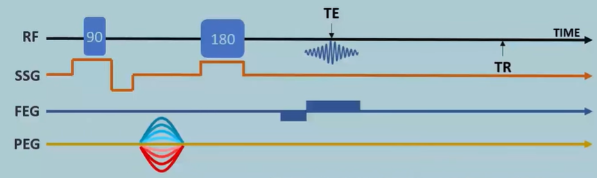
The Need for Phase Encoding: To address this limitation, phase encoding is introduced. It involves applying a gradient along the y-axis between the 90° and 180° RF pulses.
Impact of the Phase Encoding Gradient: The phase encoding gradient (PEG) does not alter the frequency of the spins but introduces a phase shift based on their y-axis position. Spins further from the gradient's null point experience a greater phase shift.
Phase Encoding and Signal Strength: Applying the PEG causes signal loss due to dephasing, with the degree of signal loss related to the strength of the applied gradient.
Multiple Phase Encoding Steps: Multiple phase encoding steps, each with a different gradient strength, are necessary to acquire enough information to localize the signal along the y-axis.
Repetition of the Sequence: Each phase encoding step requires repeating the entire pulse sequence, leading to longer acquisition times for higher y-axis resolution.
K-Space and Phase Encoding: The acquired data for each phase encoding step is stored in k-space. Each row in k-space represents the signal acquired with a specific phase encoding gradient strength.
Fourier Transform and Phase Encoding: A 1D inverse Fourier transform is applied to each row of k-space to convert the time-domain signal into a frequency-domain (x-axis location) signal.
Decoding Phase Information: The variations in signal intensity across different phase encoding steps, combined with the frequency encoded data, are used to determine the y-coordinate of the signal source.
Two-Dimensional Fourier Transform: The complete 2D spatial information (x and y coordinates) is obtained by performing a 2D inverse Fourier transform on the k-space data.
The lecture concludes by highlighting the complexity of phase encoding and encourages viewers to revisit the concepts multiple times for a thorough understanding. It emphasizes that the degree of dephasing caused by the phase encoding gradient is the key to localizing the signal along the y-axis.
Diagram Explanation
The "Diagram" image illustrates the process of acquiring and reconstructing a single horizontal line in k-space using a combination of frequency and phase encoding gradients in MRI. Here's a detailed explanation of each stage, drawing on insights from the provided YouTube sources:
Stage 1: Slice Selection
Goal: Isolate a specific slice of tissue along the z-axis of the patient. This process is not explicitly shown in the "Diagram" image, but it's a crucial preliminary step before frequency and phase encoding can occur.
Method: A slice selection gradient (SSG) is applied simultaneously with a radiofrequency (RF) pulse. The SSG creates a magnetic field gradient along the z-axis, causing protons at different z-locations to precess at different frequencies.
RF Pulse Resonance: The RF pulse is tuned to resonate with the protons in the desired slice, tipping their net magnetization vector into the transverse plane. Only the selected slice generates a detectable signal.
Rephasing Gradient:
The rephasing gradient is applied along the z-axis (slice selection direction) to correct for phase incoherence introduced by the slice selection gradient. When a slice is selected, protons across the slice thickness experience slightly different magnetic field strengths due to the slice selection gradient, causing them to precess at slightly different frequencies and leading to phase variations within the slice. The rephasing gradient, applied immediately after the slice selection gradient and RF pulse, is equal in magnitude but opposite in direction to the slice selection gradient. This effectively cancels out the phase variations by ensuring that protons across the slice thickness experience an equal and opposite magnetic field, averaging out their magnetic field exposure and bringing them back into phase. This results in a stronger, more coherent signal and helps to maintain the spatial resolution of the slice by preventing signal loss and blurring in the slice selection direction.
Apply gradient to B field to create a gradient of procession frequencies
Apply pulse for a set range of frequencies to flip the protons within that small slice
Apply a rephasing gradient to undo the frequency gradient you created. Now we have a small slice of protons that are precessing in the transverse plane, and now they all have the same frequency again as the gradient was undone and they’re only affected by the B_0 field.
Stage 2: Phase Encoding
Goal: Encode spatial information along the y-axis by introducing a phase shift to spins based on their y-position.
Method: A phase encoding gradient (PEG) is applied along the y-axis for a short period, as depicted in the "Diagram." The strength of the PEG determines the degree of phase shift experienced by spins at different y-locations.
Stronger PEG: Spins further away from the center experience a larger phase shift, leading to greater signal loss due to dephasing.
Result: This stage doesn't directly acquire signal but prepares the spins in the selected slice to be spatially encoded along the y-axis.
Stage 3: Frequency Encoding and Signal Acquisition
Goal: Encode spatial information along the x-axis and acquire the MR signal.
Method: A frequency encoding gradient (FEG) is applied along the x-axis, as shown in the "Diagram." This gradient causes protons at different x-locations to precess at distinct frequencies. The MR signal is then detected by receiver coils.
Data Acquisition: The signal is sampled multiple times during the application of the FEG. This sampling generates a series of data points that represent the net magnetization vector of the entire slice at different points in time.
(FEG Initial Dephasing described in lecture #8)
Stage 4: Storing Data in K-Space
Goal: Organize the acquired data based on the applied frequency and phase encoding gradients.
K-Space: A mathematical domain that represents the spatial frequencies of the MR image. It is essential for image reconstruction.
Data Placement: In the "Diagram," the acquired signal data, representing a single line in k-space, is positioned based on the strength of the previously applied PEG.
Each row in k-space corresponds to a specific phase encoding step.
Horizontal Location: The data points' horizontal position within the row is determined by the frequency encoding process.
Stage 5: 1D Inverse Fourier Transform
Goal: Convert the time-domain signal acquired during frequency encoding into a frequency-domain signal representing spatial information along the x-axis.
Method: A 1D inverse Fourier transform is applied to the data in the acquired k-space line.
Output: This stage generates a line of data that represents the signal intensity variations along the x-axis of the selected slice. This line, however, does not yet contain information about the y-axis location.
Stage 6: Repeating the Process
Multiple Phase Encoding Steps: To obtain a complete image, the entire sequence (Stages 1-5) is repeated multiple times with different PEG strengths. Each repetition results in a new line of data in k-space, gradually filling the entire k-space matrix.
Higher Resolution: Increasing the number of phase encoding steps increases the resolution along the y-axis but also lengthens the scan time.
Stage 7: 2D Inverse Fourier Transform
Goal: Reconstruct the complete 2D image from the fully sampled k-space data.
Method: A 2D inverse Fourier transform is applied to the k-space matrix.
Image Formation: This mathematical operation transforms the spatial frequency data back into a spatial image, where each pixel's brightness represents the signal intensity at that specific x and y coordinate.
Key Takeaways
The "Diagram" highlights how a single line in k-space is generated through a combination of slice selection, phase encoding, frequency encoding, and signal acquisition. The complete 2D image is then reconstructed by repeating this process with various phase encoding gradient strengths and finally applying a 2D inverse Fourier transform to the filled k-space matrix. The lecture emphasizes that k-space fundamentally represents the spatial frequencies of the MR image, and both frequency and phase encoding gradients contribute to sampling those frequencies. This detailed process ensures that each pixel in the final MR image accurately reflects the signal intensity at its corresponding spatial location within the patient.
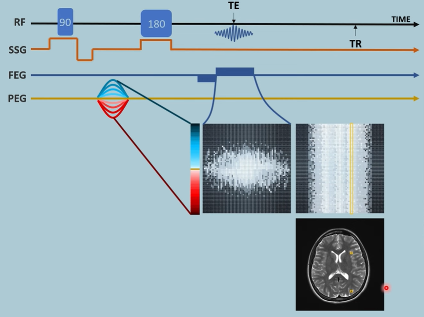
In K-Space:
x-axis is the sampling of received signal over time
y-axis is the same sampling but for shifted phases
In right diagram:
One row of the left diagram is the sampled intensities of the signal with a particular phase. This undergoes a Fourier transform and forms a row in the right diagram. Each row represents the intensities of frequencies that make up a row in the left diagram. Each frequency represents an x-coordinate in the actual slice (not the case for k-space as it is time. not space coordinates on x-axis).
Lecture Notes vs Videos
The YouTube lectures simplify the description of k-space axes, referring to them as "time" (x-axis) and "phase" (y-axis). While this provides a basic understanding, the PDF offers a more accurate and detailed explanation using the concepts of spatial frequency and phase encoding strength. Let's compare the two perspectives:
YouTube Explanation:
X-axis ("Time"): Represents the time during which the signal is acquired during the application of the frequency encoding gradient. Each point along the x-axis corresponds to a specific time point within the data acquisition window.
Y-axis ("Phase"): Represents the different phase encoding steps applied during the sequence. Each row corresponds to a unique phase encoding gradient strength.
PDF Explanation:
X-axis (Spatial Frequency u or kx): Represents the spatial frequencies encoded along the x-axis due to the frequency encoding gradient. Higher values on the x-axis correspond to higher spatial frequencies, representing finer details in the image. The PDF uses u in earlier chapters and kx in the MRI chapter to denote spatial frequencies in the x-direction.
Connection to Time: The x-axis is indirectly related to time because the spatial frequency u is proportional to the product of the frequency encoding gradient strength (Gx) and the time (t) elapsed during the readout: u = γGxt.
Y-axis (Spatial Frequency v or ky): Represents the spatial frequencies encoded along the y-axis due to the phase encoding gradient. Similarly, higher values on the y-axis correspond to higher spatial frequencies in the y-direction. The PDF uses v and ky to denote spatial frequencies along the y-axis.
Connection to Phase Encoding: The y-axis is related to the strength of the phase encoding gradient (Gy) because each row in k-space represents a different phase encoding step, which corresponds to a unique Gy value applied during the sequence.
Comparison and Key Points:
YouTube: Uses simplified terms ("time" and "phase") that relate to the pulse sequence timing and gradient application.
PDF: Emphasizes the fundamental concept that k-space represents the spatial frequencies of the MR image, using the terms u, v, kx, and ky to represent these frequencies.
Connecting the Explanations: The time-domain signal acquired during frequency encoding is converted to the frequency domain (spatial frequencies along the x-axis) through the Fourier transform. The different phase encoding steps (different Gy values) sample different spatial frequencies along the y-axis.
Central Point in K-Space: The center of k-space represents the lowest spatial frequencies (both u and v close to zero), containing information about the overall image contrast. The outer regions of k-space represent higher spatial frequencies, encoding fine details and edges.
The PDF's explanation using spatial frequencies provides a deeper understanding of how k-space relates to the final MR image, highlighting that each point in k-space represents a specific spatial frequency component of the image.