Microeconomics - VEO-Slide Bài 1+2

VIETNAM ECONOMICS OLYMPIAD

TOPIC 1: INTRODUCTION TO ECONOMICS

The Foundations of Economics

• A fundamental problem:

  • Unlimited economic wants >< Limited economic resources

• Society’s economic wants: the economic wants of its citizens and institutions.

• Economic resources: the means of producing goods and services (labor, capital, natural resources…)

What is Economics?

• Economics is the study of how a society manages its scarce resources to fulfill the needs and wants of its people.

• It is concerned with the efficient use of scarce resources to achieve the maximum satisfaction of economic wants.

Scarcity and Choice

• Scarcity: There are not enough resources to produce all the goods and services that people want.

• Choice: We “can’t have it all”, we must decide what we will have and what we must forgo.

• Opportunity cost: The opportunity cost of an item is what you give up to obtain that item. It is the next best alternative forgone.

Three Basic Economic Questions

• What to produce?

  • What types of goods and services the society chooses to produce?

• How to produce?

  • What sort of technology can be used to produce the goods and services?

• For whom to produce?

  • How the goods and services are distributed among people?

Economic Systems

• An economic system is a particular set of institutional arrangements and a coordinating mechanism.

• Economic systems differ as to

  • Who owns the factors of production

  • The method used to coordinate and direct economic activities

Economic Systems

• Market economy: an economy which is characterized by the private ownership of resources and the use of market and prices to coordinate and direct economic activities.

• Command economy: an economy in which resources are owned by government and economic decision making occurs through a central economic plan.

• Mixed economy: an economy which has the combination of features of market and command economies. The government and the private sector jointly solve economic problems.

Microeconomics and Macroeconomics

• Microeconomics looks at specific economic units. It studies the behavior of individual economic units such as consumers, firms, investors, workers … as well as individual markets.

• Macroeconomics studies the aggregate behavior of the economy. Macroeconomics seeks to obtain an overview or general outline of the structure of the economy and the relationships of its major aggregates.

Tools of Economics

• Models are simplification of the fact that omits many details to allow us to see what is truly important.

• Economic models are composed of diagrams and equations that show relationships among economic variables. “All models are wrong, but some models are useful.”

TOPIC 2: MARKET ANALYSIS

DEMAND

• Demand is the amount of some good or service consumers are willing and able to purchase at each price

• Demand schedule is a table that shows the relationship between the price of the good and the quantity demanded.

• Demand curve is a graphical presentation of the relationship between the price of the good and the quantity demanded.

Law of Demand

• The law of demand: All else equal, as price falls the quantity demanded rises and as price rises the quantity demanded falls.

Demand and Quantity Demanded

• Demand describes the behavior of a buyer at every price (i.e. the demand curve).

• Quantity demanded is a particular quantity that is demanded at a particular price.

Demand and Quantity Demanded

• A movement along the demand curve: a change in quantity demanded caused by a change in the price of the product.

Demand and Quantity Demanded

• A shift of the demand curve: a change in demand.

• Increase in demand: The demand curve shifts to the right.

• Decrease in demand: The demand curve shifts to the left.

Determinants of Demand

• Determinants of demand are factors that cause the demand curve to shift. They are also called the demand shifters. They are:

  • Consumers’ tastes and preferences

  • Consumers’ income

  • The prices of related goods

  • Expectation

  • Number of buyers

  • Weather

Income

• Normal goods: products whose demand varies directly with income.

  • As income increases (decrease) the demand for a normal good will increase (decrease).

• Inferior goods: products whose demand varies inversely with income.

  • As income increases (decrease) the demand for an inferior good will decrease (increase).

Prices of Related Goods

• Substitute goods are goods that are similar to one another and can be consumed in place of one another.

  • When the price of a good falls (rises), the demand for its substitute good decreases (increases).

• Complementary goods are goods that are consumed in conjunction with one another.

  • When the price of a good falls (rises), the demand for its complementary good increases (decreases).

SUPPLY

• Supply is the amount of a product that producers are willing and able to sell at each price.

• Supply schedule is a table that shows the relationship between the price of the good and the quantity supplied.

• Supply curve is a graphical presentation of the relationship between the price of the product and the quantity supplied.

Law of Supply

• The law of supply: All else equal, as price rises the quantity supplied rises and as price falls the quantity supplied falls.

• There is a positive or direct relationship between price and quantity supplied.

Supply and Quantity Supplied

• Supply describes the behavior of a seller at every price (i.e. the supply curve).

• Quantity supplied is a particular quantity that is supplied at a particular price.

Supply and Quantity Supplied

• A movement along the supply curve: a change in quantity supplied caused by a change in the price of the product.

Supply and Quantity Supplied

• A shift in the supply curve: a change in supply.

• Increase in supply: The supply curve shifts to the right.

• Decrease in supply: The supply curve shifts to the left.

Determinants of Supply

• Determinants of supply are factors that cause the supply curve to shift. They are also called the supply shifters. They are:

  • Resource prices

  • Technology

  • Taxes and subsidies

  • Prices of other goods

  • Expectations

  • Number of sellers

  • Weather

MARKET EQUILIBRIUM

• Market equilibrium is achieved at the price at which quantities demanded and supplied are equal.

• It is established at the intersection of demand and supply curves.

• Market equilibrium determines

  • Equilibrium price P*

  • Equilibrium quantity Q*

Market Analysis

• Market analysis: study the fluctuations in market price and quantity as a result of changes in market conditions.

• Market equilibrium changes when there is a change in market conditions.

  • Change in supply

  • Change in demand

  • Change in supply and demand

GOVERNMENT CONTROLS ON PRICES

• In a free, unregulated market system, market forces establish equilibrium prices and equilibrium quantities.

• Sometimes government believes that the market price is unfair to buyers or sellers, so government may place legal limits on prices.

• The result is government-created price ceilings and floors.

Price Ceilings and Price Floors

• Price ceiling: A legal maximum on the price at which a good can be sold.

  • Price ceiling creates a shortage.

• Price floor: A legal minimum on the price at which a good can be sold.

  • Consequences of price floor

  • Price floor creates a surplus.

ELASTICITY

• Elasticity allows us to analyze supply and demand with greater precision.

• Elasticity is a measure of how much buyers and sellers respond to changes in market conditions.

Price Elasticity of Demand

• The price elasticity of demand measures the responsiveness of quantity demanded to changes in price.

• The price elasticity of demand is computed as the percentage change in the quantity demanded divided by the percentage change in price.

• Formula for price elasticity of demand

  • $E<em>P = \frac{\frac{\Delta Q}{(Q</em>1 + Q<em>2)/2}}{\frac{\Delta P}{(P</em>1 + P_2)/2}} = \frac{\%\Delta Q}{\%\Delta P}$

  • $E_P = \frac{\Delta Q}{\Delta P} \times \frac{P}{Q} = Q' \times \frac{P}{Q}$

Price Elasticity of Demand

• Elastic Demand:

  • Percentage change in quantity demanded is greater than percentage change in price.

  • E_P > 1

• Inelastic Demand:

  • Percentage change in quantity demanded is less than percentage change in price.

  • E_P < 1

• Unit Elastic:

  • Percentage change in quantity demanded is equal to percentage change in price.

  • $E_P = 1$

• Perfectly inelastic:

  • Quantity demanded does not change as price changes.

  • $E_P = 0$

• Perfectly elastic:

  • A small percentage change in price causes an extremely large percentage change in quantity demanded.

  • $E_P = \infty$

Price Elasticity and Total Revenue

• Total revenue is the amount that a seller receives from the sale of a good.

• Total revenue is computed as the price of the good times the quantity sold.

• $TR = P \times Q$

• When demand is elastic:

  • An increase in price results in a decrease in total revenue.

  • A decrease in price results in an increase in total revenue.

• When demand is inelastic:

  • An increase in price results in an increase in total revenue.

  • A decrease in price results in a decrease in total revenue.

• When demand is unit elastic:

  • A change in price results in no change in total revenue.

Cross Price Elasticity of Demand

• Cross price elasticity of demand is a measure of the responsiveness in quantity demanded of one good to changes in the price of another good.

• It is computed as the percentage change in quantity demanded of one good (X) divided by the percentage change in the price of another good (Y).

Cross Price Elasticity of Demand

• Substitute goods: If the cross price elasticity of demand is positive then X and Y are substitute goods.

  • If E_{X,Y} > 0 → Goods are substitutes.

• Complementary goods: If the cross price elasticity of demand is negative then X and Y are complementary goods.

  • If E_{X,Y} < 0 → Goods are complement.

• Unrelated goods: If the cross price elasticity of demand is zero then X and Y are unrelated.

  • If $E_{X,Y} = 0$ → Goods are unrelated.

Income Elasticity of Demand

• Income elasticity of demand is a measure of the responsiveness in quantity demanded to changes in income.

• It is computed as the percentage change in the quantity demanded divided by the percentage change in income.

Income Elasticity of Demand

• Normal goods: Those goods that have positive income elasticity of demand.

  • Higher income raises the quantity demanded for normal goods.

• Inferior goods: Those goods that have negative income elasticity of demand.

  • Higher income lower the quantity demanded for inferior goods.

Income Elasticity of Demand

• Goods consumers regard as necessities tend to be income inelastic: E_I < 1

  • Examples include food, fuel, clothing, utilities, and medical services.

• Goods consumers regard as luxuries tend to be income elastic: E_I > 1

  • Examples include sports cars, furs, and expensive foods.

Price Elasticity of Supply

• Price elasticity of supply is a measure of the responsiveness of quantity supplied to changes in price.

• The price elasticity of supply is computed as the percentage change in the quantity supplied divided by the percentage change in price.

Price Elasticity of Supply

• Elastic supply: The price elasticity coefficient is greater than 1.

• Inelastic supply: The price elasticity coefficient is less than 1.

• Unit elastic supply: The price elasticity coefficient is 1.

• Perfectly inelastic supply: The price elasticity coefficient is zero.

• Perfectly elastic supply: The price elasticity coefficient is infinite.

TOPIC 3: THE THEORY OF CONSUMER CHOICE

Theory of Consumer Behavior

• Theory of consumer behavior: description of how consumers allocate incomes among different goods and services to maximize their well-being.

• Consumer behavior is best understood in three distinct steps:

  • Budget constraints

  • Consumer preferences

  • Consumer choices

Budget Constraints

• Budget constraint: what the consumer can afford.

• Budget constraint is the constraint that the consumers faces as a result of limited incomes.

  

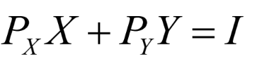
Budget Constraints

• Budget line shows all combinations of goods that can be consumed within the budget limit.

  

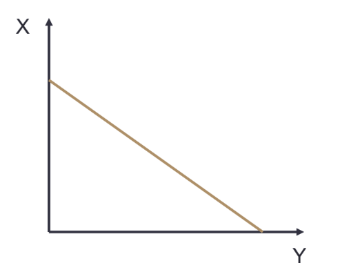
The Effects of Changes in Income and Prices

• Income changes: Shift in the budget line.

• Price changes: Change in the slope of the budget line.

Consumer Preferences

• Consumer preferences: what the consumer wants

• Basic assumptions about preferences:

  • Completeness: Consumers can compare and rank all possible market baskets (bundles) of goods.

  • Transitivity: Preferences are transitive.

  • More is better than less: More of any good is preferred to less.

Utility

• The satisfaction or pleasure one gets from consuming a good or service is called utility.

• Total utility (U) is the total amount of satisfaction a person receives from consuming a particular quantity of a good.

  • $U = U(Q)$

• Marginal utility (MU) is the additional utility a person receives from consuming one more unit of a good.

  • $MU = \frac{\Delta U}{\Delta Q}$

Law of Diminishing Marginal Utility

• The law of diminishing marginal utility: the marginal utility gained by consuming additional unit of a good will decline as more of the good is consumed.

• As Q increases, MU decreases.

Indifference Curves

• The consumer’s preferences are represented with indifference curves.

• Indifference curve: a curve that shows all combinations of goods that provide a consumer with the same level of satisfaction.

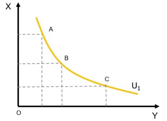
Indifference Curves

• Indifference map: a graph that contains a set of indifference curves.

The Shapes of Indifference Curves

• Marginal rate of substitution (MRS): amount of a good that a consumer is willing to give up in order to obtain one additional unit of another good (while remaining the same level of satisfaction).

• MRS is the slope of the indifference curve.

Properties of Indifference Curves

• Higher indifference curves are preferred to lower ones.

• Indifference curves are downward sloping.

• Indifference curves do not cross.

• Indifference curve are bowed inward (convex).

Consumer’s Optimal Choice

• Optimization: what the consumer chooses.

• How do consumers allocate their money incomes among different goods and services to achieve the highest level of satisfaction?

Consumer’s Optimal Choice

• Consumer’s optimal choice occurs at the tangency point of the budget constraint and the highest possible indifference curve.

Consumer’s Optimal Choice

• At the consumer’s optimal choice, the slope of the indifference curve is equal to the slope of the budget constraint.

• MRS = Price ratio of the two goods

  • $\frac{MU<em>X}{MU</em>Y} = \frac{P<em>X}{P</em>Y}$

Utility Maximization

• Utility maximizing combination of goods

• $MU<em>X/P</em>X = MU<em>y/P</em>y$

How Changes in Income Affect the Consumer’s Choices

• When income changes, the budget constraint shifts.

• Normal good: a good for which an increase in income raises the quantity demanded.

• Inferior good: a good for which an increase in income reduces the quantity demanded.

How Changes in Prices Affect the Consumer’s Choices

• A fall in the price of a good has two effects:

  • Substitution effect: Consumers tend to buy more of the good that has become cheaper and less of the good that is relatively more expensive.

    • Change in consumption of a good associated with a change in its price, with the level of utility held constant.

  • Income effect: Because one of the goods is now cheaper, consumers enjoy an increase in real purchasing power.

    • Change in consumption of a good resulting from an increase in purchasing power, with relative price held constant.

TOPIC 4: THE THEORY OF FIRM: PRODUCTION AND COSTS

What is a Firm?

• Business firm is an entity that employs factors of production (resources) to produce goods and services to be sold to consumers, other firms or the government.

The Objective of the Firm

• There are two sides to a business firm: a revenue side (total revenue) and a cost side (total cost).

• Total revenue is amount of money the firm receives from the sale of its product.

• Total cost is the costs that the firm incurs for the use of inputs.

• Profit is the difference between total revenue and total cost.

  • $\pi = TR – TC$

• The firm’s objective is to maximize its profit.

Production Function

• Production is a process of transforming inputs into output.

• Production function shows the maximum quantity of output that can be produced from a given amount of various inputs.

  • $Q = F(K, L)$

Short Run Production Relationships

• Total product (Q) is the quantity or total output of a particular good produced.

• Marginal product of labor (MPL) is the additional output that the firm can produce when it employs one more unit of labor.

  • $MPL = \frac{\Delta Q}{\Delta L}$

• Average product of labor (APL) is output per unit of labor input. It is also called labor productivity.

  • $APL = \frac{Q}{L}$

Short Run Production Costs

• In the short run, some resources (inputs) are fixed and other resources (inputs) are variable.

• Short run costs may be divided into fixed costs and variable costs.

• Fixed costs are the costs incurred for the use of fixed inputs.

• Variable costs are the costs incurred for the use of variable inputs.

Fixed, Variable and Total Costs

• Total fixed costs (TFC) are those costs that do not vary with the level of output produced.

  • Examples are rental payment, interest on firm’s debt, insurance premium.

• Total variable costs (TVC) are those costs that change with the level of output produced.

  • Examples are payments for materials, fuel, power, labor …

• Total costs (TC) is the sum of fixed costs and variable costs at each level of output.

  • $TC = TFC + TVC$

Average and Marginal Costs

• Average fixed cost (AFC) is fixed cost per unit of output

  • $AFC = \frac{TFC}{Q}$

• Average variable cost (AVC) is variable cost per unit of output

  • $AVC = \frac{TVC}{Q}$

• Average total cost (ATC) is total cost per unit of output

  • $ATC = \frac{TC}{Q}$

  • $ATC = AFC + AVC$

• Marginal Cost (MC) is additional cost that the firm incurs when it produces one more unit of output.

  • $MC = \frac{\Delta TC}{\Delta Q}$

Relation of MC to AVC and ATC

• The MC curve intersects the ATC curves at its minimum point.

  • When MC is less than ATC then if Q increases ATC will fall.

  • When MC is higher than ATC then if Q increases ATC will rise.

• The MC curve intersects the AVC curve at its minimum point.

  • When MC is less than AVC then if Q increases AVC will fall.

  • When MC is higher than AVC then if Q increases AVC will rise.

Shifts of Cost Curves

• Cost curves will shift when there is a change in

  • Taxes and subsidies

  • Input prices

  • Technology

Long Run Production Costs

• In the long run, a firm can adjust all its resources: all inputs are variable.

• In the long run, there are no fixed costs. All costs are variable costs.

• Total costs = Total variable costs

The Long Run Cost Curve

• The long run ATC curve - the firm’s planning curve - shows the lowest average total cost at any level of output produced.

• It is the envelope of all possible short run ATC curves.

Economies of Scale, Constant Economies of Scale and Diseconomies of Scale

• The long run average cost curve displays 3 regions:

  • Economies of scale: long run average total cost falls as quantity of output increases.

  • Constant returns to scale: long run average total cost is unchanged as quantity of output increases.

  • Diseconomies of scale: long run average total cost rises as quantity of output increases.

• The minimum efficient scale (MES) is the level of output at which a firm can minimize its long run average total cost.

TOPIC 5: MARKET STRUCTURES

Market Structures

• Market structure is a set of market characteristics that determines the economic environment in which a firm operates.

• It describes the competitive environment of the market.

• Market structure depends on

  • The number and relative size of firms in the industry.

  • The degree of product similarity or differentiation.

  • Conditions of entry and exit.

PERFECT COMPETITION

• Characteristics of perfect competition

  • Numerous number of small firms: There are many firms and each firm is relatively small in size.

  • Standardized product: Product is identical or homogenous.

  • Free entry and exit: There is no barriers to entry or exit the market.

  • Perfect information: Sellers and buyers have full access to information regarding the product.

  • Price taker: Each firm is a price taker. It can sell as much product as it wants at the market price. Each firm has no market power.

Demand as Seen by a Perfectly Competitive Firm

• The firm is a price taker so it can sell as much product as it wants at the market price.

• No matter how many product the firm can sell, it still receives the market price. Thus the demand for a perfectly competitive firm is perfectly elastic.

Total Revenue, Average Revenue and Marginal Revenue

• Total revenue (TR) is the amount of money that a firm receives from selling its output.

  • $TR = P \times Q$

• Average revenue (AR) is the revenue per unit of output sold.

  • $AR = \frac{TR}{Q} = P$

• Marginal revenue (MR) is the additional revenue that the firm receives when it sells one more unit of output.

  • $MR = \frac{\Delta TR}{\Delta Q} = P$

Output Decision in the Short Run

• Because a perfectly competitive firm is a price taker, it can sell as many output as it wants at the market price.

• How many output that the firm will choose to produce and sell to maximize its profit?

Profit Maximization Rule

• Marginal revenue (MR) is the revenue that the additional unit of output would add to total revenue.

• Marginal cost (MC) is the cost that the additional unit of output would add to total cost.

  • If MR > MC, firm should increase the level of output

  • If MR < MC, firm should reduce the level of output

  • If MR = MC, firm produces output level that maximizes its profit.

• Profit maximizing condition

  • MR = MC

• For a perfectly competitive firm, profit is maximized when P = MR = MC

Long Run Equilibrium

• Entry eliminates economic profits.

• Exit eliminates losses.

• Long run equilibrium is where firms earn zero economic profits

Why Do Competitive Firms Stay in Business If They Make Zero Profit?

• Total cost includes all the opportunity costs of the firm.

• In particular, total cost includes the time and money that the firm owners devote to the business.

• In the zero-profit equilibrium, the firm’s revenue must compensate the owners for these opportunity costs.

• Economic profit is zero, but accounting profit is positive.

MONOPOLY

• Characteristics of monopoly

  • Single seller: There is only one firm supplies a product for the whole market.

  • Unique product: There are no close substitutes for the product.

  • Blocked entry: strong barriers to prevent other firms to enter the market.

  • Price maker: The monopolist has the entire market power to set the price for its product.

Why Monopolies Arise

• Barriers to entry are the factors that prohibit firms from entering an industry.

• Three main sources of barriers to entry:

  • Monopoly resources: A key resource required for production is owned by a single firm

  • Government regulation: The government gives a single firm the exclusive right to produce some good or service.

  • Economies of scale: A single firm can produce output at a lower cost than can a larger number of firms.

Monopoly’s Demand and Marginal Revenue

• Total Revenue

  • $TR = P \times Q$

• Average Revenue

  • $AR = \frac{TR}{Q} = P$

• Marginal Revenue

  • $MR = \frac{\Delta TR}{\Delta Q}$

Monopoly’s Demand and Marginal Revenue

• Because a monopoly is the sole producer in the market, its demand curve is the market demand curve.

• The monopolist faces a downward-sloping demand curve.

• The monopolist’s demand and marginal revenue curves are not the same.

• At any level of output, price is higher than marginal revenue P > MR.

• The monopolist’s marginal revenue curve lies below its demand curve.

Monopoly’s Output and Pricing Decision

• What specific price-quantity combination will the monopolist choose to maximize its profit?

• The monopolist will choose the level of output where its marginal revenue equals its marginal cost. MR = MC

Monopoly’s Output and Pricing Decision

• A monopolist firm has no supply curve.

• There is only one combination of price and quantity that the monopolist chooses to supply to maximize its profit.

• At the optimal level of output

  • MR = MC

  • P > MC: The price that the monopolist charges for its product is higher than its marginal cost.

Possibility of Losses by Monopolist

• Pure monopoly does not guarantee profit.

• If demand is week and costs are high then the pure monopolist may incur loss.

Price Discrimination

• Price discrimination: a pricing practice that charges different prices for the same product.

Conditions for Price Discrimination

• Monopoly power: The seller must have the ability to control output and price.

• Market segregation: The seller must be able to segregate buyers into distinct classes, each of which has a different willingness or ability to pay for the product.

• No resale: Buyers cannot resell the product among themselves.

MONOPOLISTIC COMPETITION

• Characteristics of monopolistic competition

  • Many sellers

  • Differentiated products

  • Easy entry to and exit from the market

  • Each firm is a price maker

The Firm’s Demand Curve

• Each monopolistically competitive firm faces a downward-sloping demand curve.

• The price elasticity of demand faced by each firm depends on the number of rivals and the degree of product differentiation.

• The larger the number of rivals and the weaker the product differentiation, the greater the price elasticity of each firm’s demand.

Monopolistic Competition in the Short Run

• The monopolistically competitive firm maximizes its profit or minimizes its loss by producing at the level of output where MR = MC

• In the short run, the monopolistically competitive firm can either earn economic profit or loss.

Monopolistic Competition in the Long Run

• In the long run, firms will enter the market if it is profitable and leave the market if it is unfavorable.

  • Profits → Firms enter: Economic profits attract new firms to enter the market, demand for existing firms’ product fall and their profits decline. Economic profits are eventually driven to zero.

  • Losses → Firms leave: Losses cause some firms to leave the market, demand for existing firms’ product rise and their losses are reduced. Eventually the losses will be eliminated.

• In the long run, firms earn zero economic profit.

OLIGOPOLY

• Characteristics of oligopoly

  • A few large firms dominate the market.

  • Homogeneous or differentiated products

  • Mutual interdependence: each firm’s outcome depends not only on its own decision but also on decisions of other firms. When each firm makes decision, it has to consider the actions and reactions of other firms.

  • Significant barriers to entry

  • Each firm is a price maker

The Cartel Theory

• In a given industry, oligopolist firms will be best off if they cooperate and act as one firm. They form a cartel to act just like a monopolist to capture the maximum level of profit.

• Cartel is an organization of firms that reduces output and increases price in an effort to increase joint profits.

• Problems with cartels

  • Costly to form a cartel.

  • Difficult to reach agreement in formulating cartel policy.

  • Potential of new firms entering the industry.

  • Problem of cheating among cartel members.

Game Theory

• In oligopoly market, mutual interdependence exists among firms.

• Each firm must make strategic choice based on the consideration of actions and reactions of other firms.

• Game theory is a mathematical technique used to analyze the behavior of decision makers who try to reach an optimal position for themselves in strategic situations.

• Nash equilibrium: a set of actions for which all players are choosing their best strategies given the strategies chosen by their rivals.

Dominant Strategy

• Dominant strategy is a strategy that is best for a player in a game regardless of the strategies chosen by the other players

• Dominant strategy equilibrium is the outcome when both players have dominant strategies and play them.

• In prisoners’ dilemma, Anna and Bob both choose to confess.

• When there is no dominant strategy, each player’s strategy depends on other player’s strategy.

TOPIC 6: MARKET FAILURES AND THE ROLE OF GOVERNMENT

Market Failures

• Market failure is a circumstance in which private markets do not bring about the allocation of resources that best satisfies society’s wants.

• Three kinds of market failures:

  • Public goods

  • Externalities

  • Information asymmetries

Externalities

• Externality is a cost or a benefit accruing to a third party (bystander) that is external to a market transaction.

  • Negative externalities: impact on the third party is adverse.

  • Positive externalities: impact on the third party is beneficial.

Negative Externalities

• Negative externality creates costs to the third party which is called external costs

• Social costs will be higher than private costs

  • MSC = MPC + MEC

    • MSC: social marginal costs

    • MPC: private marginal costs (market supply)

    • MEC: marginal external costs

• The market equilibrium output is the output at which MPC = MPB

• The socially optimal output is the output at which MSC = MPB

• Consequences of negative externalities

  • Overproduction: The equilibrium market output QE is greater than the socially optimal output QO

  • This creates deadweight loss

Positive Externalities

• Positive externality creates benefit to the third party which is called external benefit.

• Social benefits will be higher than private benefits

  • MSB = MPB + MEB

    • MSB: social marginal benefit

    • MPB: private marginal benefit (market demand)

    • MEB: marginal external benefit

• The market equilibrium output is the output at which MPB = MPC

• The socially optimal output is the output at which MSB = MPC

• Consequences of positive externalities

  • Underproduction: the market equilibrium output QE is less than the socially optimal output QO

  • This creates deadweight loss

Private Solutions

• Property rights

• Moral codes and social sanctions

• Charities

• Contracts

Government Role in Externality Problem

• Solutions to positive externalities

  • Subsidies to buyers: increase demand

  • Subsidies to producers: increase supply

  • Public provision: government provides the good as a public good.

• Solutions to negative externalities

  • Regulation

  • Corrective taxes (Pigovian taxes)

  • Market for externality right

A Market for Externality Rights

• The government creates a market for externality rights.

• A pollution-control agency determines the amount of pollutants that firms can discharge into the air while maintaining the air quality at some acceptable level. The supply of pollution rights is fixed.

• The demand for pollution rights is downward sloping.

• The market determines the price for pollution rights.

Private Goods

• Private good characteristics

  • Rivalry (in consumption): one person’s use of the good diminishes other people’s use of it

  • Excludability: some people can be prevented from using the good

Public Goods

• Public good characteristics

  • Nonrivalry (in consumption): one person’s consumption of a good does not preclude consumption of the good by others.

  • Nonexcludability: there is no effective way to exclude individuals from the benefit of the good.

  • Free-rider problem: Once the good is provided everyone can obtain the benefit without payment.

Government Role in Public Goods Problem

• Since public goods have no market, they cannot be supplied privately.

• The government should provide the public goods and tax people to finance its spending.

Information Failures

• Asymmetric information: unequal knowledge possessed by the parties to a market transaction.

• Buyers and sellers do not have