Unit 8: Fiscal Policy: Multipliers, Taxes, and Government Budgetary Impacts

Fiscal Policy Unit Learning Objectives

Impact of Government Purchases on the Economy:
- Understand the mechanics of how changes in government purchases ( $G$ ) affect aggregate output ( $Y$ ).
- Ability to solve for the new equilibrium level of output following a change in government purchases.
- Identify and plot the new equilibrium on the planned expenditure ( $PE$ ) graph.
- Apply the government purchases multiplier to quantify the total impact of a change in $G$ on output.
- Demonstrate how changes in government purchases cause shifts in the Investment-Savings ( $IS$ ) curve.
Impact of Taxes on the Economy:
- Understand how changes in taxes ( $T$ ) transmit through the economy.
- Ability to solve for the new equilibrium level of output following a change in taxes.
- Identify and plot the new equilibrium on the planned expenditure ( $PE$ ) graph.
- Apply the tax multiplier to quantify the impact of a change in $T$ .
- Demonstrate how changes in taxes cause shifts in the $IS$ curve.
Balanced Budget and Automatic Stabilizers:
- Understand the economic outcome of a balanced budget change (simultaneous equal changes in $G$ and $T$ ).
- Define and identify automatic stabilizers.
- Explain the concept of the full-employment budget.
- Distinguish between a structural deficit and a cyclical deficit.

Government Purchases and equilibrium

Initial Economic Parameters (Base Case):
- Consumption: $C = 100 + 0.5(Y - T)$
- Investment: $I = 100 - 5r$
- Government Purchases ( $G$ ): $100$
- Taxes: $50$
- Real Interest Rate: $5$

Calculate Investment (I) and the Consumption (C)

(I) = 100 - 5 (5)
= 100 - 25
= 75

C =100 + 0.5 (Y - 50) =
100 + 0.5Y - 25
(100 - 25)
= 75 + 0.5Y
Use the equilibrium condition:
Y = C + I + G
Substitute the expressions for C, I, and G into the equation
Y = (75 + 0.5Y) + 75 + 100
Solve for Y: Y = 250 + 0.5Y
- Equilibrium Output (The problem solved) ( $Y$ ): Based on these parameters, the initial equilibrium output is $500$ .

Impact of Reducing Government Purchases:

Suppose they reduce government purchases, what impact does this

have on the economy?

Mechanism of Reduction: If the government reduces purchases, planned expenditure ( $PE$ ) falls, which causes the $PE$ curve to shift down.
This then causes an unplanned increase in inventory. $\left(U.I\right)$ goes up ^
Firms find themselves with unsold goods.
Firms thus respond to this unplanned increase by reducing production, so output/income falls in order to correct it.

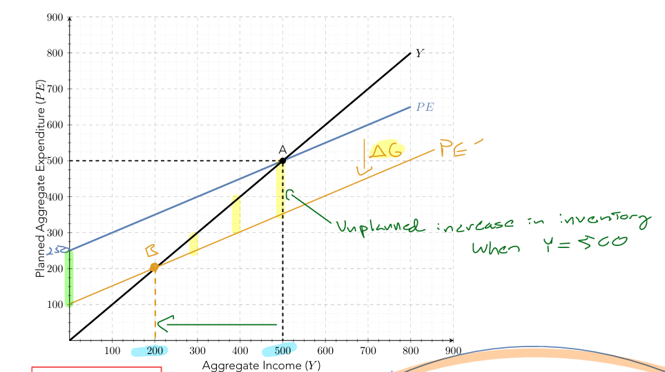
How much did government purchases fall according to our diagram: 150

How much did output fall by according to our diagram: 300 (Point B 500 - 300 = 200)

The Multiplier Effect Logic:
- Initial Change: We know that a fall in government purchases ( $\Delta G$ ) causes planned expenditure to fall initially. This means that firms are accumulating unplanned inventory.
- First Round: Firms see an unplanned increase in inventory, so they cut production. This reduced production would cause income to fall.
- Second Round and Beyond: The fall in income causes consumption ( $C$ ) to fall by the amount of the Marginal Propensity to Consume ( $MPC$ ) multiplied by the change in income ( $\Delta C = MPC \times \Delta Y$ ). This fall in consumption leads to a further fall in planned expenditure.
- Cycle Completion: Firms again see unplanned inventory increases, further reduce production, and further reduce income/consumption. This cycle continues until the economy reaches a new equilibrium (Point B on the graph).
- Summary: The fall in government purchases results in lower income, causing repeated falls in consumption, which means that output will fall by more than the initial change in government purchases.

Quantifying the Government Purchases Multiplier:
- The change in output ( $\Delta Y$ ) relative to the change in government purchases ( $\Delta G$ ) is determined by the multiplier.
- Multiplier Formula: $\text{Multiplier} = \frac{1}{1 - MPC}$
- MPC Influence: An increase in the $MPC$ will increase the size of the multiplier. This occurs because the multiplier effect is driven by the relationship between income and consumption; the larger the $MPC$ , the larger the impact that each successive change in income has on consumption.
- Numerical Example from Transcript:
  - Initial Output ( $Y^*$ ): $500$
  - Change in Government Purchases ( $\Delta G$ ): $-150$
  - $MPC$ : $0.5$
  - Multiplier calculation: $\frac{1}{1 - 0.5} = \frac{1}{0.5} = 2$
  - Change in Output ( $\Delta Y$ ): $2 \times (-150) = -300$
  - New Equilibrium Output ( $Y'$ ): $500 - 300 = 200$

Government Purchases and the IS Curve

Dynamics on the Planned Expenditure Graph:
- A fall in government purchases causes the planned expenditure line to shift down.
- This results in a fall in the equilibrium level of output in the goods market.
Relationship with Interest Rates:
- If the interest rate ( $r$ ) remains fixed (e.g., at $r=5$ ), the fall in $G$ directly reduces output.
Shifting the IS Curve:
- The $IS$ curve represents the combinations of interest rates and income levels where the goods market is in equilibrium.
- Since the equilibrium level of output falls while the interest rate remains the same, the $IS$ curve shifts to the left.
- Following the shift, at the same interest rate ( $r_1$ ), the new equilibrium level of output ( $Y_2$ ) is lower than the original ( $Y_1$ ).

Impact of Taxes on Economics

Dynamics of Tax Reduction:
- Suppose the government reduces taxes ( $T$ ).
- Consumption Impact: A reduction in taxes increases disposable income ( $Y - T$ ), which causing consumption ( $C$ ) to rise.
- Expenditure Shift: As consumption rises, planned expenditure ( $PE$ ) rises, shifting the $PE$ curve up.
- Inventory and Production: This causes an unplanned decrease in inventory. Firms respond by increasing production, leading to a rise in total output and income ( $Y$ ).
The Tax Multiplier:
- There is a specific formula to calculate the change in output based on a change in taxes.
- Tax Multiplier Formula: $\text{Tax Multiplier} = -\frac{MPC}{1 - MPC}$
- Differences from the Government Multiplier:
  1. Negative Sign: There is an inverse relationship; a decrease in taxes causes output to go up.
  2. Numerator ( $MPC$ vs. $1$ ): The tax multiplier uses the $MPC$ in the numerator because taxes affect expenditure indirectly through consumption, whereas government purchases affect planned expenditure directly.
Taxes and the IS Curve:
- A reduction in taxes causes the planned expenditure line to shift up and output to increase.
- Assuming the interest rate does not change, the $IS$ curve shifts to the right.
- Result: At interest rate $r_1$ , the equilibrium level of output increases from $Y_1$ to $Y_2$ .

Balanced Budget and Combined Productivity Impacts

Scenario 1: Change in Government Purchases Only:
- Initial State: $G=100, T=50, MPC=0.5, Y=500$
- Change: $\Delta G = -50$
- Multiplier: $2$
- Impact: $\Delta Y = 2 \times (-50) = -100$
- New equilibrium: $Y' = 400$
Scenario 2: Change in Taxes Only:
- Change: $\Delta T = -50$
- Tax Multiplier: $-\frac{0.5}{1 - 0.5} = -1$
- Impact: $\Delta Y = -1 \times (-50) = +50$
- New equilibrium: $Y' = 550$
Scenario 3: Balanced Budget Change (Simultaneous Changes):
- Conditions: Both government purchases and taxes are decreased by the same amount ( $\Delta G = -50$ and $\Delta T = -50$ ).
- Calculation: Total change is the sum of the individual impacts.
- Total Change: $\Delta Y = -100 + 50 = -50$
- New equilibrium: $Y' = 500 - 50 = 450$
- General Principle: If both $G$ and $T$ change, the total impact on output is the algebraic sum of the two individual multipliers' effects.

The Economy’s Influence on the Government Budget

Automatic Stabilizers:
- Definition: These are revenue and expenditure items in the federal budget that automatically adjust with the state of the economy to stabilize GDP without requiring new legislation.
- Examples:
  - Unemployment Insurance: Payments increase during downturns, supporting consumption.
  - Progressive Income Tax: As incomes fall during a recession, people move into lower tax brackets, reducing the tax burden and softening the blow to disposable income.
  - Fiscal Drag: The negative effect on the economy when average tax rates increase during an expansion because taxpayers move into higher income brackets, naturally slowing down an overheating economy.
  - Social Assistance: Programs like Medicaid and food stamps enroll more people during economic downturns.
Full-Employment Budgets:
- Definition: The state of the federal budget if the economy were producing at the full-employment level of output.
- Structural Deficit: The portion of the budget deficit that remains even when the economy is at full employment. This is caused by permanent fiscal policy choices.
- Cyclical Deficit: The portion of the deficit that occurs specifically because the economy is in a downturn (reduced tax revenue and increased stabilizer spending).

Questions & Discussion

Question: Why did output fall by more than the fall in government purchases?
- Response: The initial fall in $G$ causes planned expenditure to fall. Firms accumulate unplanned inventory and cut production ( $Y$ ). As income falls, consumption falls (determined by the $MPC$ ). This secondary fall in consumption reduces planned expenditure again, leading to further production cuts. This cycle repeats until the total fall in output is a multiple of the initial change in $G$ .