Pearson's Product-Moment Correlation Coefficient & Spearman's Rank-Order Correlation Coefficient
Definition (#f7aeae)
Important (#edcae9)
Extra (#fffe9d)
Test of Normality for Correlation:
Correlation analysis assumes that the data for both variables are normally distributed.
If the data is not normally distributed, it can lead to inaccurate or misleading correlation results.
Tests for Normality:
Shapiro-Wilk Test:
Commonly used for testing the normality of a variable’s distribution.
Null hypothesis: Data is normally distributed.
If p-value is greater than 0.05, the data is normally distributed.
If p-value is less than 0.05, the data is not normally distributed.
Kolmogorov-Smirnov Test:
Tests how closely a sample matches a normal distribution.
Similar to Shapiro-Wilk, a p-value greater than 0.05 suggests normality.
Sample size less than 50: Shapiro-Wilk.
Sample size more than 50: Kolmogorov-Smirnov.
Analysis: Test of normality
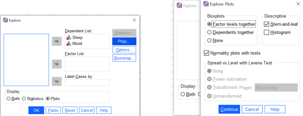
Analyse → Descriptive Statistics → Explore.
Put all variables in “Dependent List”
Click “Plots” → Tick “Normality plots with tests” → Click “continue”.
Click “OK”
Interpretation:
Kolmogorov-Smirnov or Shapiro-Wilk test not significant (p > .05).
Data is normally distributed.
Use parametric test.
Kolmogorov-Smirnov or Shapiro-Wilk test significant (p < .05).
Data is not normally distributed.
Use non-parametric test.
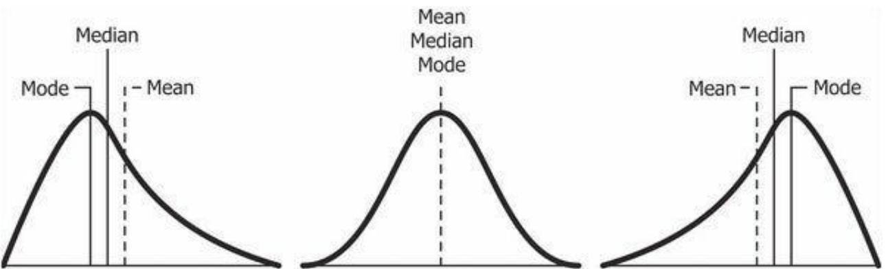
Skewness:
Tells us about the symmetry of a distribution.
Shows whether the data is leaning more to one side.
If skewness = 0, the data is perfectly symmetrical (a normal distribution).
Types:
Postive skew:
Tail is longer on the right side.
More scores are concentrated on the left.
Negative skew:
Tail is longer on the left side.
More scores are concentrated on the right.
Importance in correlation:
Pearson’s correlation assumes both variables have a normal (symmetrical) distribution.
High skewness can affect the accuracy of the correlation.
If data is skewed, consider using Spearman’s correlation instead.
Rules:
0: Perfectly normal (symmetrical) distribution.
-0.5 to 0.5: Considered approximately symmetric or normal.
0.5 to 1 (or -0.5 to -1): Moderate skew. It still can be acceptable depending on the context.
Greater than 1 (or less than -1): High skew, meaning the data is clearly skewed and less normal.
Kurtosis:
Refers to the “peakedness” or “flatness” of a distribution.
If kurtosis = 0, it’s close to a normal distribution.
Positive kurtosis: The distribution has thicker tails and a sharper peak than normal, meaning there are more extreme values.
Negative kurtosis: It has thinner tails and a flatter peak.
Rules:
Kurtosis between -1 and +1 is generally acceptable for most analyses that assume normality.
Kurtosis values beyond +/-2 indicate a distribution that is likely not normal and may require transformation or other statistical adjustments.
Like with skewness, Spearman’s correlation is preferred when normality is violated.
Handling outliers:
Use a robust measure of central tendency - Mean.
Winsorize the data, replace with the nearest values thata re not outliers.
Exclude the outlier. (With justification)
Use non parametric tests.
Cronbach’s alpha:
Measure of internal consistency.
Tells us how well a set of items measure the same underlying construct.
Values range from 0-1.
Above 0.9: Excellent.
0.8 - 0.9: Good.
0.7 0.8: Acceptable.
0.6 - 0.7: Questionable.
Below 0.6: Poor.
Importance:
Ensures that the survey/scale items work together as a group.
Tells us whether the items are reliable or consistent.
Helps improve the quality of psychological instruments.
When to use:
After developing or using likert type scale.
Before doing analysis, to check if the items are reliable.
Pearson’s Product-Moment Correlation Coefficient:
Overview:
Measures the strength and direction of the linear relationship between 2 continuous variables.
Widely used statistics to explore associations between variables such as test scores, behaviors, and traits.
Symbol: r.
Values range from -1 to +1.
Assumptions:
Both variables should be continuous and approximately normally distributed.
A linear relationship exists between the variables.
No significant outliers.
Independence of observations.
Spearman's Rank-Order Correlation Coefficient:
Overview:
A non -parametric measure of the strength and direction of association between 2 ranked or ordinal variables.
Values range from -1 to +1.
Use when data is ordinal or not normally distributed.
Relationship is not linear, but still consistent in direction.
Ranks are used instead of raw scores.
Useful for small samples or non-parametric data.
Assumptions:
Variables should be at least ordinal.
Monotonic relationship (as one increases, the other tends to increase or decrease).
Doesn’t require normality.
Less sensitive to outliers.
Analysis: Correlation
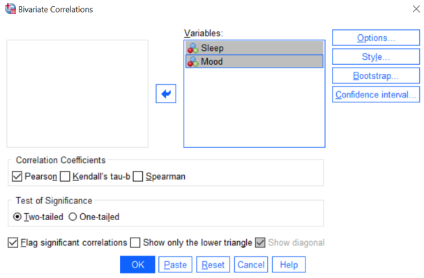
Analyze → Correlate → Bivariate.
Put variables in “Variables”.
Tick either “Pearson” or “Spearman” for “correlation coefficient” → Click “OK.
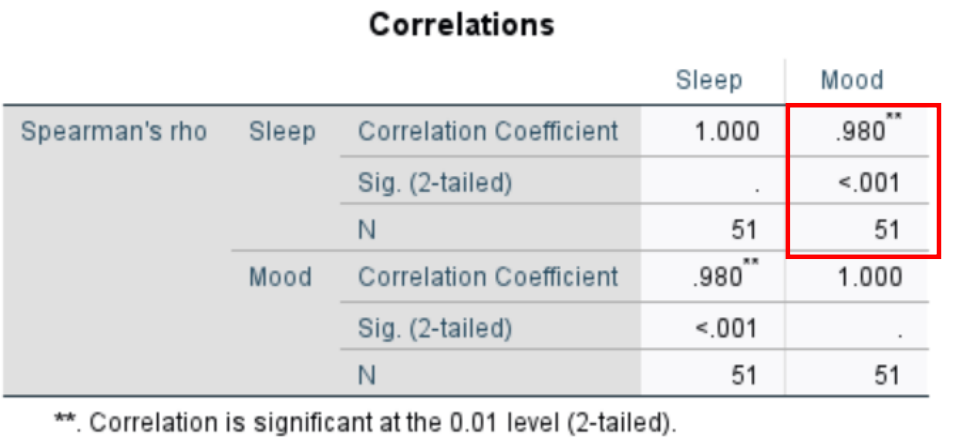
Template:
What test you ran and why & what variables were plugged in.
Is there a significant relation between the variables.
Direction and strength.
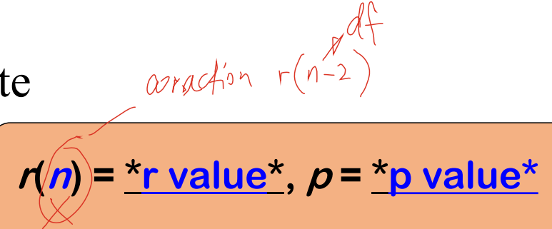
Report the “equation” above with the values.
Interpretation:
If significant: When one variable increases, what happened to the other.
If not significant: No relation.