Lecture - 8: Radiation Shielding, Build-up Factors, and Source Geometries

Energy Deposition and Exposure Rate Units

$E_d = \varphi \left( \frac{\mu_{en}}{\rho} \right)_a E_\gamma$

For this lecture take $I = \varphi$

• When analyzing radiation interaction, energy deposition is normalized to define the exposure rate.

• The energy required to ionize one kilogram of air is quantified in terms of the energy deposition rate ($\dot{X}$).

$\dot{X} = \frac{I E \left( \frac{\mu_a}{\rho} \right)_{\text{air}}}{5.47 \times 10^{7}}$

• The conversion factor for ionization is approximately $1.83 \times 10^{-8}$.

$\dot{X} = 1.83 \times 10^{-8} \, I E \left( \frac{\mu_a}{\rho} \right)_{\text{air}} \; [\text{R/s}]$

• The standard exposure rate is typically measured in milliroentgens per hour ($mR/hr$).

• The relationship between Roentgen per second and Roentgen per hour is given by:

   $1 \, \text{R/s} = 3.6 \times 10^{6} \, \text{mR/hr}$

• The exposure rate ($X$) can be calculated using the constant $0.0659$. The general formula involving energy levels ($E$), flux ($\phi$), and the mass absorption coefficient ($\frac{\mu_a}{\rho}$) is:

    $\dot{X} \space (mR/hr) = 0.0659 \times E \times I \times \left(\frac{\mu_a}{\rho}\right)$

• For environments with multiple energy levels, the exposure rate is the summation of the rates for each individual energy level:

    $\dot{X}_{total} = \sum (0.0659 \times E_i\times I_{i} \times \frac{\mu_{ai}}{\rho})$

• Total exposure over time can be determined by integrating the exposure rate. If the flux is substituted with fluence, the total exposure relative to the fluence can be calculated.

$X_{total} = \int \dot{X} \, dt$

Numerical: Intensity and Gamma Photon Flux Calculations [5:30]

How many 2‑MeV gamma rays must strike each square centimeter every hour in order to produce an exposure rate of 1 mR/hr in air?

• Example Calculation (2 MeV Gamma Photons):

  • Required mass attenuation coefficient for air ($\frac{\mu_a}{\rho}$) is $0.0238\,cm^2/g$.

  • The flux ($I$) is calculated as:

        $I = \frac{1\,mR/hr}{0.0659 \times 2\,MeV \times 0.0238} \approx 319\,\text{gamma photons}/cm^2/s$

                This assumes the value of $\frac{\mu}{\rho}$ for air is around $5\,cm^2/g$

Theoretical Foundations of Build-up Factors [8:23]

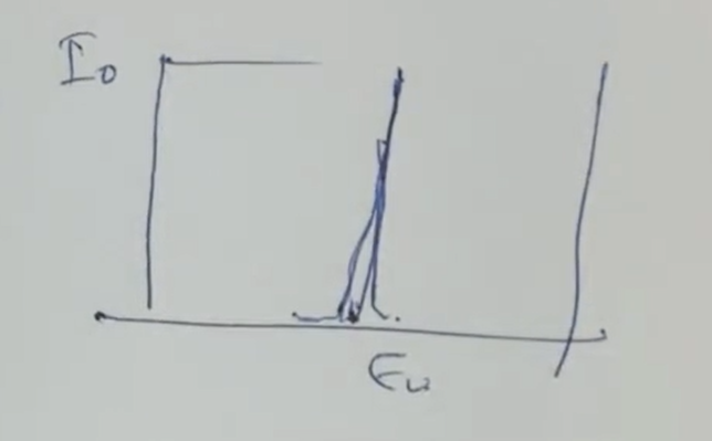
• In a situation where monoenergetic parallel beam radiation interacts with shielding material, a detector placed directly in front of the source (without shielding) records a sharp energy peak.

• After the radiation passes through shielding, the recorded spectrum changes. While a portion of the original energy remains (the uncollided flux), a continuous lower-energy spectrum also appears. This phenomenon is caused by:

  

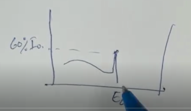
  • Compton scattering (primary contributor).

  • Photoelectric effect (resulting in X-ray emission).

  • Fluorescence.

• The radiation impacting the matter is not entirely absorbed; Compton scattered photons emerge at different energies, creating a "build-up" of radiation intensity beyond what is predicted by simple exponential attenuation.

• To account for this spread without performing complex energy-dependent integrations (which are difficult for hand calculations), the Build-up Factor ($B$) is introduced.

• The actual exposure rate behind a shield is modified by the build-up factor:

• Exposure rate before shield:

$\dot{X_o} = 0.0659 \times E \times \phi_{o} \times \left(\frac{\mu_a}{\rho}\right)$

• Exposure rate beyond the shield (Actual):

$0.0659 \int_{0}^{E_0} \phi(\varepsilon)\,E\left(\frac{\mu_a}{\rho}\right)^{\text{air}}\, d\varepsilon$

• Simplified:

$\dot{X_u} = \dot{X_o} \times B(\mu a) \times e^{-\mu \times a}$

• The buildup factor is a function of $\mu \times a$, where:

  • $\mu$ is the linear attenuation coefficient.

  • $a$ is the thickness of the shielding or distance traveled.

  • The product $\mu \times a$ represents the number of mean free paths, or the number of scattering events the radiation undergoes through the material thickness.

$\mu \times a = \frac{1}{\lambda} \times a$

Tabulated Build-up Factors

• Build-up factors are categorized based on source geometry and are found in standard tables:

  • Table 10.1: Exposure build-up factors for mono-directional sources (beam radiation).

  • Table 10.2: Exposure build-up factors for isotropic point sources.

• The build-up flux ($\phi_B$) can be expressed as the product of the initial flux ($\phi_o$) and the build-up factor ($B$), often denoted as $B_m$ for mono-directional sources:

    $\phi_b = \phi_{o} \times B(\mu a) \times e^{-\mu \times a}$

 $\phi_b = \phi_{u} \times B(\mu a)$

Numerical Problem: Mono-directional Beam through Lead Shielding [21:40]

A monodirectional beam of 2‑MeV gamma rays has an intensity of
10⁶ photons per square centimeter per second.

This beam strikes a lead (Pb) sheet that is 10 centimeters thick.

At the rear side of the lead shield, calculate the following:

1. Uncollided flux

2. Buildup flux

3. Exposure rate

Use the following data:

• The mass attenuation coefficient of lead at 2 MeV is
  $\left(\frac{\mu}{\rho}\right)_{\text{Pb}} = 0.0457\ \text{cm}^2/\text{g}$

• The mass attenuation (Check) coefficient of air at 2 MeV is:
  $\left(\frac{\mu}{\rho}\right)_{\text{air}} = 0.0238\ \text{cm}^2/\text{g}$

• The density of lead is:
  $\rho_{Pb} = 11.34\ \text{g/cm}^3$

Part (a) solution:

• Step 1: Calculate Linear Attenuation ($\mu$):

    $\mu = 0.0457 \times 11.34 = 0.518\,cm^{-1}$

• Step 2: Calculate Uncollided Flux ($\phi_u$):

    $\phi_u = \phi_0 \times e^{-\mu x} = 10^6 \times e^{-(0.518 \times 10)} = 10^6 \times e^{-5.18}$     $\phi_u \approx 5.63 \times 10^3\,photons/cm^2.s$

Part (b) solution:

• Step 3: Determine Build-up Factor ($B_m$) at $\mu x = 5.18$:

  • Using interpolation from Table 10.1 for $2\,MeV$: At $\mu x = 4$ ($B = 2.41$) and $\mu x = 7$ ($B = 3.36$):

  • Slope for interpolation: $\frac{3.36 - 2.41}{7 - 4} = 0.3167$

$B_{5.18} = 2.41 + 0.3167 \times (5.18 - 4) \approx 2.784$

• Step 4: Calculate Build-up Flux:

    $\phi_B = (5.63 \times 10^3) \times 2.78$

$= 1.56 \times 10^4\,photons/cm^2/s$

Part (c) solution:

• Step 5: Calculate Exposure Rate:

$\dot{X_b} = 0.0659 \times E \times \phi_{} \times \left(\frac{\mu_a}{\rho}\right)$

$\dot{X_b} = 0.0659 \times 2 \times 1.56 \times 10^4 \times 0.0238$

$= 48.8 \hspace{0.2cm} mR/h$

Point Source Calculations and Shield Design [29:20]

• For an isotropic point source ($S$ ) emitting radiation in all directions, the uncollided flux at distance $r$ is:

    $\phi_u = \frac{S}{4 \pi r^2} e^{-\mu r}$

• The build-up flux ($\phi_B$) is calculated using the point source build-up factor ($B_p$):

    $\phi_B = B_p(\mu r) \times \frac{S}{4 \pi r^2} e^{-\mu r}$

Numerical Problem: Spherical Iron Shielding [31:00]:

An isotropic point source emits 108 photons every second. Each photon has an energy of 1 MeV. You want to surround this source with a spherical iron shield.

Your goal is to determine how large the radius of the shield must be so that the exposure rate measured at the outer surface of the shield is only 1 mR/hr.

You are given the following data:

• The mass energy‑absorption coefficient of air at 1 MeV is

      $\left( \frac{\mu_a}{\rho} \right)_{\text{air}} = 0.0280\ \text{cm}^2/\text{g}$

• The mass attenuation coefficient of iron at 1 MeV is        $\left( \frac{\mu}{\rho} \right)_{\text{Fe}} = 0.0595\ \text{cm}^2/\text{g}$

• The density of iron is

        $\rho_{\text{Fe}} = 7.86\ \text{g/cm}^3$

Graphical Solution Method:

$\dot{X_b} = 0.0659 \times E \times \phi_b \times \left(\frac{\mu_a}{\rho}\right)$

$\phi_b = \frac{\dot{X}}{0.0659\,E\left( \frac{\mu_a}{\rho} \right)^{\text{air}}}$

$= \frac{1}{0.0659\,E\left( \frac{\mu_a}{\rho} \right)^{\text{air}}}$

$= 542~\text{photons}\,/\,\text{cm}^2\cdot\text{s}$

$\mu = \left(\frac{\mu}{\rho}\right)\rho = 0.0595 \times 7.86 = 0.468\ \text{cm}^{-1}$

• Multiplu neumerator and denominator by $\mu²$:

 $\phi_B = B_p(\mu r) \times \frac{S}{4 \pi r^2} e^{-\mu r}$

$542 = \frac{10^{8}\, B_{p}(\mu R)\, e^{-\mu R}}{4\pi R^{2}}$

• Take RHS

$1 = \frac{3219.65\, B_p(\mu R)\, e^{-\mu R}}{(\mu R)^2}$

• Since $r$ is unknown in both the exponent and the build-up factor, the equation is solved by assuming various values for $\mu r$ (e.g., 2, 4, 6) and calculating the corresponding right-hand side of the equation.

• By plotting these values and finding where they equate to the desired flux, a specific $\mu r$ is determined.

• For this problem, the calculated $\mu r$ is approximately $6.55$.

• Required Radius: $r = \frac{6.55}{0.468} \approx 14\,cm$.

Analytical Expressions: Taylor and Berger Forms [42:07]

• Build-up factors can be expressed analytically instead of using tables.

• Taylor Form: Represented as a sum of two exponential terms for point sources:

    $B(\mu r) = A_1 e^{-\alpha_1 μ r} + A_2 e^{-\alpha_2 μ r}$

• Constraint: $A_1 + A_2 = 1$.

• Tables providing $A_1$, $α_1$, and $α_2$ allow for calculating the second constant$A_2$.

• Berger (or Dietz) Form: An alternative analytical expression given as:

    $B = 1 + C(\mu r) e^{D μ r}$

Specific Radiation Source Configurations [45:00]

• Line Source (Infinite):

  • For an infinitely long line source ($S$) at distance $x$:

$d\phi_r(P) = \frac{S\,dz}{4\pi r^2}$

$\text{Total flux} = \int d\phi_r = \frac{S}{4\pi} \int_{-\infty}^{\infty} \frac{dz}{r^2}$

$r^2 = x^2 + z^2$        

$\phi = \frac{S}{4\pi} \times \int_{-\infty}^{\infty} \frac{dz}{x^2 + z^2}$

Using the identity $\int \frac{1}{x^2 + a^2} dx = \frac{1}{a} \tan^{-1}(\frac{x}{a})$

$= \frac{S}{4\pi}\,\left.\left|\frac{1}{x}\,\tan^{-1}\!\left(\frac{z}{x}\right)\right|\right|_{-\infty}^{\infty}$

        $\phi = \frac{S}{4x}$

• Line Source (Finite Length):

  • For a source with length segments $L_1$ and $L_2$:

        $\phi = \frac{S}{4 π x} [\tan^{-1}(\frac{L_2}{x}) + \tan^{-1}(\frac{L_1}{x})]$

• Ring Source:

  • For a ring of radius $R$ with the detector at distance $x$ from the center:

$d\phi(P) = \frac{s\,dl}{4\pi r^2}$        

$\phi = \frac{SR}{2 r^2}$, where $r^2 = x^2 + R^2$

• Disc Source:

  • Calculated by considering a disk as a series of rings with radius $z$ and differential width $dz$.

• The total flux involves integration across the disk radius $R$:

        $\phi = \frac{S}{4} \ln(1 + \frac{R^2}{x^2})$

Infinite Plane Sources and Exponential Integrals [58:00]

• For infinite plane sources, the flux calculation involves the Exponential Integral Function ($E_n$).

• The uncollided flux from an infinite plane source is given by:

    $\phi_u = \frac{S}{2} E_1(\mu r)$

• The first-order exponential integral function ($E_1(x)$) is defined as:

    $E_1(x) = \int_x^{\infty} \frac{e^{-t}}{t} dt$

• When build-up is included using the Taylor form, the total build-up flux becomes a sum of exponential integral functions:

    $\phi_B = \frac{S}{2} \sum A_n E_1(\mu r [1 + \alpha_n])$

Questions & Discussion

May be added later.