DASC 120 Week 6 Lecture 6.1 Two Sample Proportion Testing
Formal HT (Hypothesis Testing): limitations and conditions
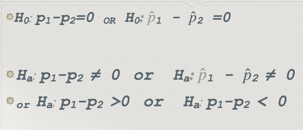
If the null hypothesis is true, the difference between the two population proportions would be the null value, 0.5.
The sampling distribution of phat be normal when two conditions are met:
Independence: the data come from two independent random samples or if the data come from a randomized experiment
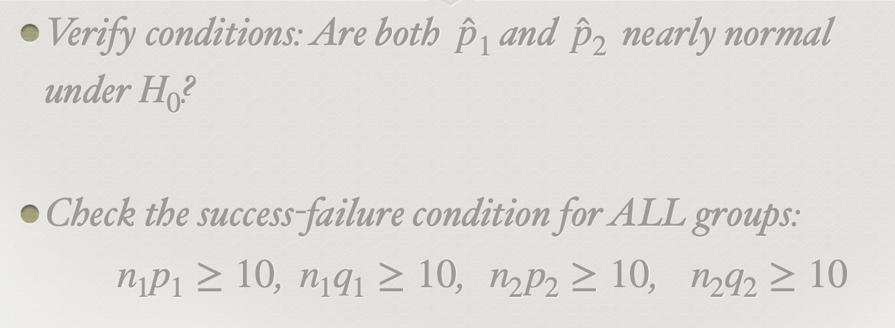
Success-Failure

Once we have demonstrated that it is appropriate to use this test
(Ie: Supported by the Central Limit Theorem for the Sampling Distribution of the Null)
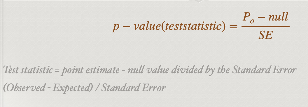
We compare the p value to our alpha value:

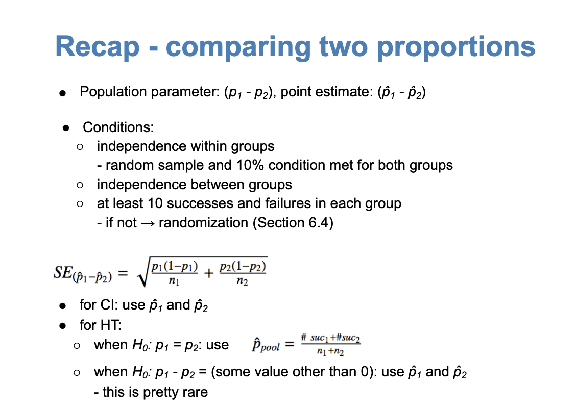
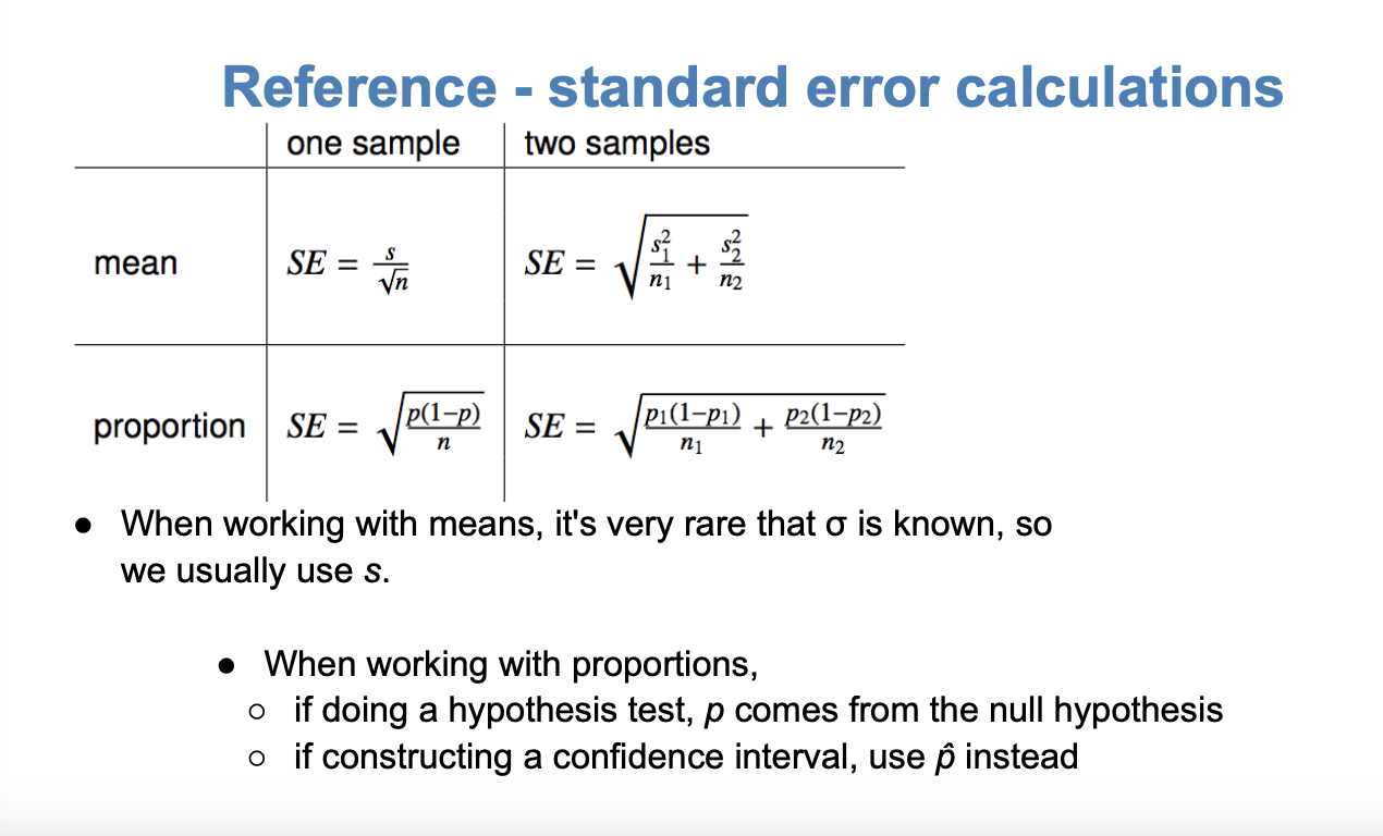
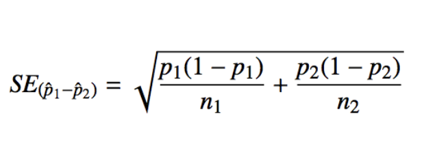
Standard Error for the difference in two proportions
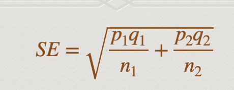
For each of the two samples, first find the proportion of "success" (what we are want) for each group. Then find the "failures" (the observations that were not what we wanted) for each group.
Multiply successes x failures, and divide by total number of observations for each group.
Add them together and take the square root.
Confidence intervals for the difference in two proportions
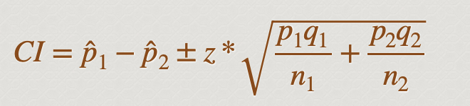
Point estimate ± z* (SE) —> to find the range, multiply the Z the matches our confidence level by the standard error. The lower value is the point estimate minus this value; the upper is the point estimate plus this value
Parameter of interest (population parameter) could be
Proportion of all people in a group
Difference between two proportions of all of each group
etc
ALWAYS P
Point estimate could be
Proportion of a sample of a group
Difference between two proportions of the sample of each group
etc
ALWAYS PHAT
Standard error of the difference between two SAMPLE proportions
Conditions for CI for difference of proportions
1. Independence within groups:
Groups are sampled randomly
sample < 10% of the population
if the sample is less than 10% of the total population, it’s unlikely that people’s responses are dependent on each other
2. Independence between groups:
The sampled groups are independent of each other
3. Success-failure:
At least 10 observed successes and 10 observed failures in the two groups.
Sample proportions are also nearly normally distributed
You determine that sample proportions are nearly normally distributed by verifying that each group has at least 10 expected successes and 10 expected failures. This confirms that the sampling distribution follows an approximately normal shape.
Pooled estimate of a proportion
In the case of comparing two proportions where H0: p1 = p2, there isn't a given null value we can use to calculated the expected number of successes and failures in each sample.
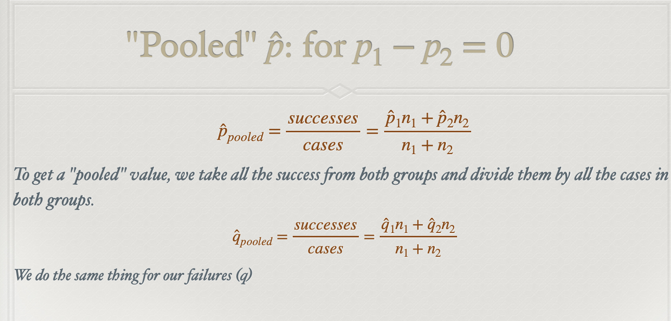
Therefore, we need to first find a common (pooled) proportion for the two groups, and use that in our analysis.
This simply means finding the proportion of total successes among the total number of observations.