AP Calculus AB Unit 1 (Limits): Notation, Estimation, Algebraic Techniques, Strategy, and the Squeeze Theorem

Defining Limits and Using Limit Notation

What a limit is (the core idea)

Calculus is built on the concept of the limit. Unlike Algebra, where we usually compute exactly what a function equals at a specific point, calculus asks a different question: what value does the function approach as we get closer and closer to a specific input?

A limit describes what value a function’s output is approaching as the input gets close to a particular number. The key word is approaching: a limit is about what happens near a point, not necessarily at the point.

Formally, we write:

\lim_{x \to a} f(x) = L

This is read: “The limit of %%LATEX1%% as %%LATEX2%% approaches %%LATEX3%% equals %%LATEX4%%.” (Many textbooks also use %%LATEX5%% instead of %%LATEX6%%; the idea is identical.)

Why limits matter

Limits are the foundation for two of the biggest ideas in calculus.

Derivatives are defined using a limit of an average rate of change as the input change shrinks toward zero. Definite integrals are built from limits of sums as the rectangle width shrinks toward zero. When you learn limits, you’re learning the language calculus uses to describe “getting arbitrarily close.”

Limit value vs. function value (journey vs destination)

It is crucial to understand that the function value and the limit value can be different.

• The function value is %%LATEX7%%, what happens exactly at %%LATEX8%%.
• The limit %%LATEX9%% is what happens for %%LATEX10%% values close to a.

The value %%LATEX12%% does not determine the limit. The point %%LATEX13%% might be undefined (a hole), or it might be defined at a different height; the limit only cares about the journey as you approach a, not the destination.

Two-sided limits and one-sided limits

A two-sided limit looks at approaching from both directions:

\lim_{x \to a} f(x)

A one-sided limit looks from only one direction:

\lim_{x \to a^-} f(x)

\lim_{x \to a^+} f(x)

• %%LATEX18%% means values less than %%LATEX19%% moving up toward a (from the left).
• %%LATEX21%% means values greater than %%LATEX22%% moving down toward a (from the right).

Existence Theorem (two-sided limit):

\lim_{x \to a} f(x) = L \text{ exists if and only if } \lim_{x \to a^-} f(x) = \lim_{x \to a^+} f(x) = L

If the left-hand and right-hand limits are different, then the two-sided limit does not exist (DNE).

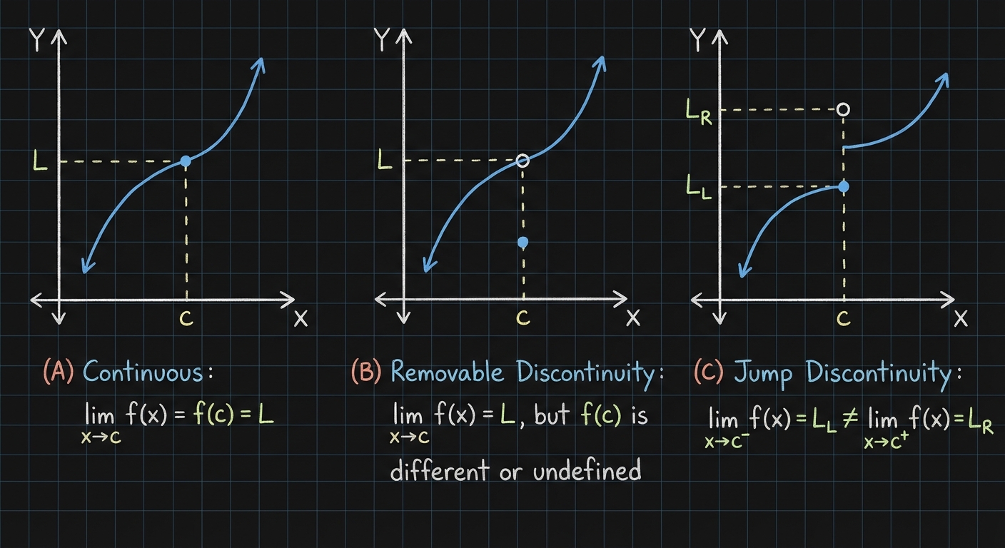
When limits fail to exist

A limit can fail to exist for a few common reasons:

1. Jump discontinuity: the left and right sides approach different values.
2. Infinite behavior (vertical asymptote): the function grows without bound.
3. Oscillation: the function keeps bouncing around without settling to one value (for example, expressions involving %%LATEX25%% near %%LATEX26%%).

Notation reference (what the symbols mean)

Worked example 1: Limit exists but function value differs

Suppose a function behaves like

f(x)=\frac{x^2-1}{x-1}

for %%LATEX36%%, so it is not defined at %%LATEX37%%. Even so, we can ask what value %%LATEX38%% approaches as %%LATEX39%%.

Factor the numerator:

x^2-1=(x-1)(x+1)

So for x \ne 1,

f(x)=\frac{(x-1)(x+1)}{x-1}=x+1

Now take the limit using the simpler expression:

\lim_{x \to 1} f(x)=\lim_{x \to 1} (x+1)=2

Even though f(1) is undefined, the limit exists and equals 2.

Worked example 2: Two-sided limit does not exist because sides disagree

Imagine that as %%LATEX45%% approaches 3 from the left, %%LATEX46%% approaches 1, but from the right it approaches 5:

\lim_{x \to 3^-} f(x)=1

\lim_{x \to 3^+} f(x)=5

Because 1 and 5 are different,

\lim_{x \to 3} f(x) \text{ DNE}

Exam Focus

• Typical question patterns:
  • “Evaluate \lim_{x \to a} f(x)” and justify using left- and right-hand behavior.
  • “Does the limit exist? Explain” using one-sided limits or a graph.
  • Interpret a statement like \lim_{x \to 2} f(x)=7 in words.
• Common mistakes:
  • Confusing %%LATEX52%% with %%LATEX53%% (especially when there is a hole).
  • Claiming a two-sided limit exists without checking both sides.
  • Mixing up %%LATEX54%% and %%LATEX55%% (left vs right).

Estimating Limit Values from Graphs and Tables

How to read a limit from a graph (finger-tracing method)

Before using algebra, you must be able to visually and numerically estimate limits.

A graph is often the fastest way to see a limit. To estimate %%LATEX56%% from a graph, locate %%LATEX57%% on the horizontal axis and trace the curve toward a from both sides. Many students literally “trace with your fingers” from the left and from the right.

• Continuous path: if your two traces meet, the limit is the y-value where they meet.
• Holes (removable discontinuity): if your traces meet at an open circle, the limit exists and is the y-value of the hole.
• Jumps: if your traces approach different heights, the limit is DNE.
• Vertical asymptotes: if the graph shoots up to infinity or down to negative infinity, the two-sided limit does not exist as a real number (because infinity is not a real number), but you should still describe the behavior as approaching %%LATEX61%% or %%LATEX62%% when appropriate.

A powerful point: the limit depends on the curve near %%LATEX63%%, not on whether there’s a filled dot at %%LATEX64%%. The dot affects f(a), not the limiting behavior.

One-sided limits from graphs

Graphs make one-sided limits very concrete.

• For %%LATEX66%%, only look at the part of the graph with %%LATEX67%% as it approaches a.
• For %%LATEX69%%, only look at the part of the graph with %%LATEX70%%.

This is especially important for piecewise-defined functions, where the rule can change at x=a.

Vertical asymptotes and infinite limits

Sometimes, as %%LATEX72%% approaches %%LATEX73%%, the outputs grow without bound. You may see the graph shooting upward or downward near a vertical line.

In that case, you describe the behavior with an infinite limit, such as:

\lim_{x \to a} f(x)=\infty

or

\lim_{x \to a} f(x)=-\infty

This does not mean the limit exists as a real number; it means the function increases or decreases without bound.

Estimating limits from a table

Tables give numerical evidence of a limit by showing values of %%LATEX76%% for inputs close to %%LATEX77%%. A good table:

• Approaches a from both sides.
• Uses values increasingly close to a.

You are not looking for exact equality; you are looking for a trend: do the outputs settle toward a single number?

Worked example 1: Estimating from a table (approaches 4)

Suppose you want \lim_{x \to 2} f(x) and you are given:

From the left, values move toward about 4. From the right, values also move toward about 4. So you would estimate:

\lim_{x \to 2} f(x)=4

Worked example 2: Estimating from a table (approaches 5)

To estimate \lim_{x \to 2} f(x), you might see a table like this, with values approaching 2 from both sides:

Observation: as %%LATEX89%%, %%LATEX90%% approaches 5, so:

\lim_{x \to 2} f(x)=5

Worked example 3: Estimating one-sided limits from a graph (typical scenario)

Imagine a graph where:

• As %%LATEX92%%, the curve approaches %%LATEX93%%.
• As %%LATEX94%%, the curve approaches %%LATEX95%%.

Then:

\lim_{x \to 1^-} f(x)=2

\lim_{x \to 1^+} f(x)=-1

So:

\lim_{x \to 1} f(x) \text{ DNE}

What can go wrong with tables

Tables can mislead if:

• The function approaches a value slowly and rounding hides the trend.
• The function oscillates near the point.
• You only look from one side and miss a jump.

Because of this, AP questions often pair tables with prompts like “estimate” or “justify,” and they may ask for one-sided limits explicitly.

Exam Focus

• Typical question patterns:
  • Estimate %%LATEX99%% from a table; sometimes also ask for %%LATEX100%% and \lim_{x \to a^+} f(x).
  • Use a graph to determine whether a limit exists and, if so, its value.
  • Identify infinite limits from a graph near a vertical asymptote.
• Common mistakes:
  • Using the value shown at x=a (a filled dot) instead of the approached value.
  • Only checking one side of a.
  • Assuming “getting large” means “limit equals a large number” instead of recognizing \infty behavior.

Determining Limits Using Algebraic Properties and Manipulation

Why algebra helps

Graphs and tables build intuition, but calculus often needs exact results. Algebraic methods let you compute limits precisely, especially when direct substitution leads to an indeterminate form like \frac{0}{0}.

The basic limit laws (algebraic properties)

When limits exist and are finite, they follow predictable rules. If

\lim_{x \to a} f(x)=L

and

\lim_{x \to a} g(x)=M

then:

• Sum:

\lim_{x \to a} (f(x)+g(x))=L+M

• Difference:

\lim_{x \to a} (f(x)-g(x))=L-M

• Constant multiple:

\lim_{x \to a} (c f(x))=cL

• Product:

\lim_{x \to a} (f(x)g(x))=LM

• Quotient (if M \ne 0):

\lim_{x \to a} \frac{f(x)}{g(x)}=\frac{L}{M}

• Power (integer n):

\lim_{x \to a} (f(x))^n=L^n

• Root (when defined):

\lim_{x \to a} \sqrt[n]{f(x)}=\sqrt[n]{L}

• Composite functions (requires continuity of the outside function at the limiting value):

\lim_{x \to a} f(g(x))=f\left(\lim_{x \to a} g(x)\right)

Direct substitution (when it works)

Always try direct substitution first. For many functions, limits can be found by plugging in %%LATEX118%%. This works especially well for continuous functions such as polynomials, trigonometric functions like sine and cosine, and exponential functions like %%LATEX119%%.

Example 1 (polynomial):

\lim_{x \to 3} (x^2-5x+1)

Polynomials are continuous everywhere, so substitute directly:

\lim_{x \to 3} (x^2-5x+1)=3^2-5(3)+1=9-15+1=-5

Example 2 (polynomial):

\lim_{x \to 3} (x^2+2x)=(3)^2+2(3)=9+6=15

Indeterminate form and algebraic manipulation

If direct substitution gives \frac{0}{0}, that is not the answer. It is a signal that simplification is needed.

Two of the most common manipulations in AP Calculus AB limits are:

1. Factoring and canceling
2. Rationalizing with a conjugate

Factoring and canceling

Example:

\lim_{x \to 2} \frac{x^2-4}{x-2}

Direct substitution gives \frac{0}{0}. Factor the numerator:

x^2-4=(x-2)(x+2)

For x \ne 2,

\frac{x^2-4}{x-2}=x+2

Now the limit is straightforward:

\lim_{x \to 2} (x+2)=4

The cancellation is valid because limits care about values near 2, and the simplified expression matches the original for all nearby %%LATEX130%% except at the single point %%LATEX131%%.

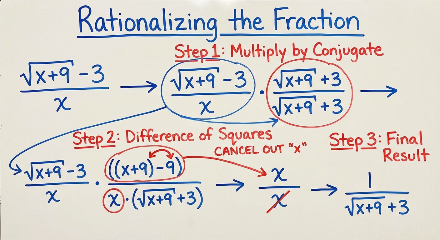
Rationalizing (using conjugates)

Rationalizing is useful when radicals create \frac{0}{0}.

Example 1:

\lim_{x \to 9} \frac{\sqrt{x}-3}{x-9}

Multiply by the conjugate:

\frac{\sqrt{x}-3}{x-9} \cdot \frac{\sqrt{x}+3}{\sqrt{x}+3}=\frac{x-9}{(x-9)(\sqrt{x}+3)}

Cancel %%LATEX135%% (for %%LATEX136%%) to get:

\frac{1}{\sqrt{x}+3}

Now substitute:

\lim_{x \to 9} \frac{1}{\sqrt{x}+3}=\frac{1}{6}

Example 2 (same idea, different setup):

\lim_{x \to 0} \frac{\sqrt{x+9}-3}{x}

Multiply numerator and denominator by the conjugate \sqrt{x+9}+3. This clears the radical and typically allows you to cancel the factor causing the zero in the denominator.

Trigonometric limits (facts you use)

In AP Calculus AB, you frequently use special trigonometric limit facts as x \to 0.

Core facts:

\lim_{x \to 0} \frac{\sin(x)}{x}=1

\lim_{x \to 0} \frac{\tan(x)}{x}=1

Also commonly used:

\lim_{x \to 0} \frac{1-\cos(x)}{x}=0

Example:

\lim_{x \to 0} \frac{\sin(5x)}{x}

Rewrite to create the form \frac{\sin(u)}{u}:

\frac{\sin(5x)}{x}=5 \cdot \frac{\sin(5x)}{5x}

Then:

\lim_{x \to 0} 5 \cdot \frac{\sin(5x)}{5x}=5 \cdot 1=5

Common misconception: canceling incorrectly

You can only cancel common factors, not terms separated by addition or subtraction.

For example, you cannot simplify

\frac{x+1}{x}

by “canceling” the x inside the sum. Always look for common factors.

Exam Focus

• Typical question patterns:
  • Evaluate a limit that produces \frac{0}{0} and requires factoring or rationalizing.
  • Use limit laws to break a complex expression into simpler limits.
  • Use the composite-function idea when a continuous outer function wraps an inner expression.
  • Compute trigonometric limits by rewriting into a known special limit form.
• Common mistakes:
  • Treating \frac{0}{0} as 0 or as “the limit doesn’t exist” without trying algebra.
  • Canceling terms instead of factors.
  • Forgetting to check denominator conditions when using quotient properties.

Selecting Procedures for Determining Limits

Why “procedure choice” is a skill

On exams (and in real problem solving), the main challenge is often not doing the algebra but deciding which tool fits the situation. A good strategy begins with recognizing what kind of expression you have and what happens under direct substitution.

A decision process you can apply

When asked to evaluate

\lim_{x \to a} \text{(expression in } x\text{)}

you can choose a method by following this logic.

Step 1: Try direct substitution

Compute the expression at x=a.

• If you get a real number, that is often the limit.
• If you get \frac{0}{0}, you need simplification.
• If you get a “nonzero divided by zero” form (like %%LATEX156%% or %%LATEX157%%), you are likely seeing vertical asymptote behavior.

Scenario A: Nonzero divided by zero (vertical asymptote behavior)

If substitution gives a nonzero numerator over 0:

• The limit does not exist as a finite real number.
• There is a vertical asymptote at that input value.
• The function may approach %%LATEX158%%, %%LATEX159%%, or approach different infinities from each side.

On AP-style questions, it is often best to state the infinite behavior when it is clear (for example, “approaches \infty”), rather than only writing DNE with no description.

Scenario B: Indeterminate form

If you get

\frac{0}{0}

then stop and simplify. This form does not mean “undefined” or “zero.” It means “we don’t know yet; more work is required.” Very often, it indicates a removable discontinuity (a hole).

Step 2: If you got \frac{0}{0}, identify the structure

Common structures and matching tools:

• Rational function with polynomial pieces: factor and cancel.
• Radical expressions: multiply by a conjugate.
• Complex fraction: combine into a single fraction (common denominator) and simplify.
• Trig expression near 0 involving sine or tangent: rearrange into special trig limit forms.
• Piecewise function at a boundary: compute one-sided limits.

Step 3: If simplification is not straightforward, consider a theorem

If you cannot easily simplify but you can trap the function between two simpler functions with the same limit, use the Squeeze Theorem.

Example 1: Choosing factoring vs direct substitution

Evaluate:

\lim_{x \to 1} \frac{x^3-1}{x-1}

Direct substitution gives \frac{0}{0}, so simplify. Recognize a difference of cubes:

x^3-1=(x-1)(x^2+x+1)

Then for x \ne 1,

\frac{x^3-1}{x-1}=x^2+x+1

Now substitute:

\lim_{x \to 1} (x^2+x+1)=1+1+1=3

This is a classic “pattern recognition” limit: difference of squares, difference of cubes, and factoring by grouping appear often.

Example 2: Choosing conjugates

Evaluate:

\lim_{x \to 4} \frac{\sqrt{x}-2}{x-4}

The radical suggests conjugates:

\frac{\sqrt{x}-2}{x-4} \cdot \frac{\sqrt{x}+2}{\sqrt{x}+2}=\frac{x-4}{(x-4)(\sqrt{x}+2)}

So the expression simplifies (for x \ne 4) to:

\frac{1}{\sqrt{x}+2}

Now substitute:

\frac{1}{\sqrt{4}+2}=\frac{1}{4}

Example 3: Recognizing an infinite limit

Evaluate:

\lim_{x \to 2} \frac{1}{(x-2)^2}

As x \to 2, the denominator approaches 0, and the square keeps it positive, so the expression grows without bound:

\lim_{x \to 2} \frac{1}{(x-2)^2}=\infty

A common mistake is to write only DNE without describing the infinite behavior. On AP-style questions, writing \infty communicates the correct idea: the outputs increase without bound.

Real-world connection: “approaching” in measurements

Limits mirror measurement and modeling: increasing precision gets you closer and closer to a value without instantly achieving perfection. Limits formalize that “closer and closer” reasoning so you can do exact mathematics with it.

Exam Focus

• Typical question patterns:
  • Multi-part questions asking you to evaluate a limit and explain your method choice (factor, conjugate, trig limit, one-sided analysis).
  • Problems where direct substitution gives either \frac{0}{0} (simplify) or nonzero over 0 (vertical asymptote behavior).
  • Limits involving piecewise definitions where one-sided limits determine existence.
• Common mistakes:
  • Sticking with direct substitution even after getting \frac{0}{0}.
  • Saying “DNE” for a vertical asymptote case without describing whether it approaches %%LATEX180%% or %%LATEX181%%.
  • Choosing conjugates when simple factoring works (or vice versa), creating unnecessary complexity.
  • Ignoring domain restrictions (for example, assuming a square-root expression behaves the same on both sides when it may not be defined).

Squeeze Theorem

What the Squeeze Theorem says

The Squeeze Theorem (also called the Sandwich Theorem) is used when a function is hard to analyze directly but can be trapped between two easier functions.

If there are functions %%LATEX182%% and %%LATEX183%% such that, for all %%LATEX184%% near %%LATEX185%% (except possibly at a),

g(x) \le f(x) \le h(x)

and

\lim_{x \to a} g(x)=L

and

\lim_{x \to a} h(x)=L

then the middle function must also approach L:

\lim_{x \to a} f(x)=L

Why it works (intuition)

Think of %%LATEX192%% as being “pinned” between two walls that are closing in on the same height. If the lower wall and the upper wall both approach height %%LATEX193%% as you approach %%LATEX194%%, there’s nowhere else for %%LATEX195%% to go.

Visual: Think of f(x) as a car being forced to drive between two guardrails; if the guardrails squeeze together toward the same height, the car’s path is forced there too.

This theorem is especially useful when:

• The function oscillates but with shrinking amplitude.
• The expression is messy but can be bounded using a known inequality.

A key inequality used frequently

A classic bounding fact is:

-1 \le \sin(x) \le 1

Similarly,

-1 \le \cos(x) \le 1

Multiplying by a nonnegative expression preserves the inequality direction, which is often how you create squeezes.

Worked example 1: A standard oscillation squeeze

Evaluate:

\lim_{x \to 0} x \sin\left(\frac{1}{x}\right)

Since \sin\left(\frac{1}{x}\right) oscillates, direct approaches do not help. Use bounding.

Start with:

\left|\sin\left(\frac{1}{x}\right)\right| \le 1

Multiply by |x|:

|x|\left|\sin\left(\frac{1}{x}\right)\right| \le |x|

Recognize:

|x|\left|\sin\left(\frac{1}{x}\right)\right|=\left|x\sin\left(\frac{1}{x}\right)\right|

So:

0 \le \left|x\sin\left(\frac{1}{x}\right)\right| \le |x|

As x \to 0, both outer limits go to 0, so the middle goes to 0. Therefore:

\lim_{x \to 0} x \sin\left(\frac{1}{x}\right)=0

Worked example 2: Squeeze with cosine

Evaluate:

\lim_{x \to 0} x^2 \cos\left(\frac{1}{x}\right)

Because

-1 \le \cos\left(\frac{1}{x}\right) \le 1

multiply by x^2 (always nonnegative):

-x^2 \le x^2\cos\left(\frac{1}{x}\right) \le x^2

Both outer limits are 0 as x \to 0, so the middle is squeezed to 0:

\lim_{x \to 0} x^2 \cos\left(\frac{1}{x}\right)=0

What goes wrong (common pitfalls)

• Incorrect bounds: If your “upper” and “lower” functions do not actually stay above and below f(x) near the point, you cannot squeeze.
• Bounds approach different limits: If %%LATEX215%% and %%LATEX216%% approach different values, the theorem gives no conclusion.
• No neighborhood: The inequality must hold for %%LATEX217%% sufficiently close to %%LATEX218%% (not necessarily for every real number).
• Sign mistake: Multiplying an inequality by a negative expression reverses the inequality signs; forgetting this breaks the argument.

Exam Focus

• Typical question patterns:
  • Prove a limit equals 0 using bounds like -1 \le \sin(x) \le 1.
  • Evaluate limits of oscillating expressions such as products involving %%LATEX220%% or %%LATEX221%%.
  • Justify a limit by explicitly naming bounding functions and showing their limits match.
• Common mistakes:
  • Forgetting to show the inequality that traps f(x) (writing only the final conclusion).
  • Multiplying an inequality by a negative expression and failing to reverse inequality signs.
  • Choosing bounds that are not tight enough to force a single limit value.