Comprehensive Guide to Statistical Sampling and Data Visualisation
Foundations of Statistical Sampling
Core Definition and Purpose:
Sampling is the method of collecting data from a subset of individuals or units selected from a larger population.
Its primary objective is to obtain empirical insights that accurately reflect the characteristics, behaviors, or parameters of the entire population without conducting a full census.
Key Rationales for Sampling Over Full Enumeration:
Time Constraints: Large populations make census data collection highly time-consuming. A sample can be acquired, processed, and analyzed within an operational, reasonable timeframe.
Financial Cost: The monetary expenditures required to track, contact, and survey every single unit in an extensive population are frequently prohibitive.
Physical Impossibility of Total Identification: Completely identifying and accessing every member of a target population can be practically impossible (e.g., conducting surveys among unhoused or transient populations who cannot be fully located or listed in a directory).
Destructive Testing Procedures: In manufacturing and quality assurance, testing certain items requires their total destruction (e.g., establishing the operating lifetimes of lightbulbs). Testing the entire population would destroy the entire inventory, making sampling mathematically and operationally indispensable.
Sources of Bias in Sampling
Sample Representativeness:
A representative sample accurately and proportionally mirrors the underlying population being studied.
Due to random sampling variation, distinct samples drawn from the same population naturally yield slightly different results because each sample comprises a different set of individuals.
When a sample fails to mirror the population, it is classified as biased.
When multiple samples are drawn and consistently deviate from the true population value in the same direction, the sampling scheme possesses systematic bias.
Taxonomy of Sampling Bias:
Selection Bias:
The systematic tendency of a sampling frame or method to include or exclude specific segments of a population.
Example: Utilizing a telephone directory as a sampling frame produces selection bias because individuals with unlisted numbers, mobile-only users, or households without fixed landlines are systematically excluded.
Non-Response Bias:
Occurs when a significant proportion of selected participants fail to return surveys or respond to inquiries.
Bias emerges because responders and non-responders frequently possess fundamentally different demographic or behavioural characteristics, skewing observed distributions.
Example: In postal or mail-in surveys, response rates are historically depressed among both low-income and high-income households, resulting in a sample that systematically over-represents middle-income households.
Response Bias:
Occurs when participants supply inaccurate, distorted, or untruthful answers.
Contributing mechanisms include poor question wording leading to misunderstandings, interviewer demeanor or bias influencing responses, and social desirability bias or privacy concerns surrounding sensitive topics (e.g., disclosing illegal activity or exact personal income).
Inherently Biased Sampling Methods:
Volunteer Sampling:
Participants self-select into the study (e.g., readers choosing whether to respond to a printed magazine questionnaire).
Attracts individuals with extreme opinions, strong motivations, or surplus leisure time, rendering the resulting sample non-representative.
Convenience Sampling:
Researchers select the most readily accessible individuals within the population (e.g., stationing an interviewer at a shopping center for a few hours).
Excludes members of the population not present at that specific time and location, resulting in localized sampling distortion.
Probability Sampling Methods and Implementations
Principles of Unbiased Sampling:
Eliminates human discretion and researcher subjectivity in picking individual sample units.
Ensures that every member of the target population possesses a known, non-zero probability of being selected.
Simple Random Sampling (SRS):
Designed to choose members from a population of size .
Key Properties:
Every individual unit in the population has an equal probability of being selected.
Every possible combination or subset of size has an equal probability of being chosen.
Practical Execution: Implemented using algorithmic computer-based pseudorandom number generators.
Demonstration with :
Selecting integers between and across three independent computational iterations:
Sample A:
Sample B:
Sample C:
Stratified Random Sampling:
The population is partitioned into non-overlapping, mutually exclusive, and exhaustive sub-populations termed strata.
Every single individual belongs to one and only one stratum.
A simple random sample is independently drawn from within each individual stratum.
Proportional Stratification: Strata are sampled in proportion to their actual share of the total population (, where is stratum size, is total population size, and is total desired sample size).
Demonstration (, across five color-coded strata):
Stratum 1 (Red): . Proportion requires units. Random draw yields: .
Stratum 2 (Blue): . Proportion requires units. Random draw yields: .
Stratum 3 (Yellow): . Proportion requires units. Random draw yields: .
Stratum 4 (Green): . Proportion requires units. Random draw yields: .
Stratum 5 (Purple): . Proportion requires unit. Random draw yields: .
Cluster Sampling:
The population is divided into pre-existing, naturally occurring groups or clusters (typically structured around geographic boundaries or administrative units).
Rather than sampling individuals across all groups, a subset of entire clusters is chosen at random.
Every single individual residing within the selected clusters is completely enumerated and surveyed.
Demonstration: A population partitioned into geographic clusters. Two clusters are selected at random ( and ); all members inside Cluster 3 and Cluster 2 constitute the final sample.
Methodological Classification Case Study (Hospital Discharge Survey in Kent):
Scenario: Measuring patient treatment satisfaction across hospitals in Kent discharged over the preceding year.
Design A: Group patients by length of hospital stay ( days, days, days, and days) and execute an SRS within each duration bracket.
Classification: Stratified Random Sampling; Unbiased.
Design B: Assign all discharged patients a unique index number and employ a computer random number generator to select the sample.
Classification: Simple Random Sampling; Unbiased.
Design C: Mount an informational flyer on hospital notice boards requesting discharged patients to complete an online feedback form.
Classification: Volunteer Sampling; Biased.
Design D: An interviewer positions themselves outside a hospital main exit for 3 hours, surveying leaving patients.
Classification: Convenience Sampling; Biased.
Design E: Utilize regional postcodes to segment Kent into geographic clusters, select a random subset of postcodes, and survey every patient discharged from the hospitals situated within those selected postcodes.
Classification: Cluster Sampling; Unbiased.
Empirical Evaluation: The Clusterville Study
Study Architecture:
Clusterville is a defined municipal study system containing households (indexed through ).
Research Objective: Select a sample of households to calculate an estimator for the population mean household annual income ().
True Population Mean: .
Spatial and Postcode Configuration:
The municipality contains 10 distinct postcodes following the format
CV1 ABn, with exactly 5 houses per postcode:CV1 AB1: HousesCV1 AB2: HousesCV1 AB3: HousesCV1 AB4: HousesCV1 AB5: HousesCV1 AB6: HousesCV1 AB7: HousesCV1 AB8: HousesCV1 AB9: HousesCV1 A10: Houses
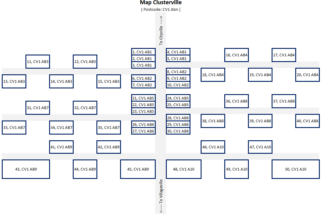
Complete Clusterville Household Income Census ():
House 1: | House 2: | House 3: | House 4: | House 5:
House 6: | House 7: | House 8: | House 9: | House 10:
House 11: | House 12: | House 13: | House 14: | House 15:
House 16: | House 17: | House 18: | House 19: | House 20:
House 21: | House 22: | House 23: | House 24: | House 25:
House 26: | House 27: | House 28: | House 29: | House 30:
House 31: | House 32: | House 33: | House 34: | House 35:
House 36: | House 37: | House 38: | House 39: | House 40:
House 41: | House 42: | House 43: | House 44: | House 45:
House 46: | House 47: | House 48: | House 49: | House 50:
Single-Trial Execution of the Four Sampling Schemes:
Convenience Sampling Implementation:
The surveyor travels south from Cityville and samples the first 10 homes encountered along the route (Houses through ).
Selected Incomes: .
Computation: .
Mean:
Bias: Substantially underestimates the population mean () because houses near Cityville contain lower-income households.
Simple Random Sampling Implementation:
Ten houses chosen purely at random: Houses .
Selected Incomes: .
Computation: .
Mean:
Cluster Sampling Implementation:
Random selection selects two postcodes: Postcode
CV1 AB2() and PostcodeCV1 AB9().All households within both clusters are sampled (Houses and Houses ).
Selected Incomes: .
Computation: .
Mean:
Stratified Sampling Implementation:
Households are divided into two physical strata based on structural footprint: Small houses (represented by smaller joined boxes: Houses and , total ) and Large houses (larger separate boxes: Houses and , total ).
Proportional allocation requires: small houses and large houses.
Small house draws: House (), House (), House (), House ().
Large house draws: House (), House (), House (), House (), House (), House ().
Computation: .
Mean:
Computational Replication and Method Performance (100 Iterations):
When each sampling procedure was executed across computer-generated iterations, the mean of the sample means demonstrated clear differences in accuracy and variability:
Convenience Sampling: Mean of means = . Classified as the worst method due to severe systematic selection bias.
Simple Random Sampling: Mean of means = . Unbiased; closely aligns with the true population parameter ().
Cluster Sampling: Mean of means = . Unbiased; converges near the true population mean.
Stratified Random Sampling: Mean of means = . Unbiased and produced the lowest standard deviation across the 100 runs. By controlling for the structural covariate (house size) linked to income, it minimized sampling variance, making it the statistically superior approach.
Application Problem (University Student Satisfaction):
When designing a study with a sample constraint of drawn from a university student population, an optimal design utilizes stratified random sampling across academic faculties and study levels (undergraduate vs. postgraduate) to ensure proportional representation, preventing under-representation of smaller academic departments.
Principles of Data Visualisation
Definition and Core Scope:
Data visualisation is the graphical representation of information and quantitative data.
It utilizes visual encodings (charts, graphs, plots, diagrams, and maps) to offer an accessible, rapid way of identifying patterns, shifts, distributions, clusters, and anomalous outliers in multidimensional data.
Early Evolution:
2nd Century CE: Emergence of structured tabular arrangements to organize numerical values, representing the earliest systematic attempt to summarize complex information.
17th Century: René Descartes formulated the Cartesian coordinate system, establishing the geometric foundation for spatial representations of quantitative coordinates ().
Historical Pioneers of Statistical Graphics
William Playfair (1759–1823):
Recognized as the founder of statistical graphics.
Invented the line chart, the bar chart, and is credited with creating the area chart and pie chart.
The Commercial and Political Atlas (1786): Contained the first published time-series line plot illustrating commercial trade between England and foreign partners (Denmark and Norway) from to .
Enclosed the area between the import and export lines to explicitly depict trade balance: an area representing "Balance against England" (trade deficit) and an area representing "Balance in Favour of England" (trade surplus).
Introduced the first bar chart, displaying Scottish export and import totals by trade partner from Christmas 1780 to Christmas 1781.
Statistical Breviary (1801): Featured the earliest recorded pie chart, visually dissecting the proportions of the Ottoman/Turkish Empire situated across Asia (), Africa, and Europe.

Florence Nightingale (1820–1910):
Acclaimed for nursing service during the Crimean War and for her role as an innovative statistician and data journalist.
Recognized through careful military hospital record-keeping that British soldiers were predominantly dying from preventable infectious diseases (zymotic diseases) caused by poor sanitation and malnutrition rather than combat wounds.
Engineered the "coxcomb", "rose diagram", or "polar area chart":
Segments the circle into equal angular wedges representing the months of the year (April 1854 to March 1856).
Area of each color-coded wedge (measured from the common center) corresponds to mortality rates: blue/gray wedges represent deaths from preventable/mitigable zymotic diseases, red wedges represent deaths from battlefield wounds, and black wedges denote all other causes.
Proved highly effective for displaying seasonal, cyclical time patterns, successfully prompting systemic hospital sanitation reforms.

John Snow (1813–1858):
London physician and founding pioneer of modern epidemiology.
Investigated the 1854 cholera outbreak in Soho, London, which had claimed over 600 lives.
Plotted the precise spatial locations of cholera fatalities directly onto a street map of the district, using stacked tally lines parallel to street frontages to represent death counts at each address.
Revealed a sharp spatial concentration surrounding the Broad Street public water pump, demonstrating waterborne disease transmission and prompting authorities to remove the pump handle to halt the outbreak.

Charles Joseph Minard (1781–1870):
French civil engineer celebrated for thematic cartography and flow mapping.
Created the famous 1869 figurative map of Napoleon's Russian campaign of 1812–1813:
Displays six variables on a single two-dimensional plane: army size, geographic distance, direction of movement, temperature, geographic location, and dates.
Utilizes a flow line (Sankey diagram style) whose width represents the size of the army (), showing the catastrophic reduction from soldiers crossing the Niemen into Russia down to reaching Moscow, and ending with just freezing survivors returning.
Linked directly to an aligned lower line graph illustrating freezing winter temperatures using the Réaumur scale (dropping to ).
Produced an 1858 economic map of France displaying the provenance of butcher cattle, calves, and sheep sent on the hoof to feed Paris, using localized pie charts whose areas were proportional to meat volume.

Edmond Halley (1656–1742):
English astronomer and geophysicist (famed for computing the orbit of Halley's comet).
Developed the cartographic use of contour lines (isolines/isopleths) to connect geographic regions possessing equal physical or atmospheric values (such as magnetic variation and barometric pressure), which form the basis for modern synoptic weather maps.
Charles de Fourcroy (1766–1824):
French mathematician and engineer.
Published the Tableau Poléométrique in 1782, a visual demographic analysis of major European cities.
Employed nested, proportional geometric squares to depict urban land areas and demographics, directly prefiguring modern hierarchical treemaps.

Luigi Perozzo (1856–1916):
Italian statistician and mathematician.
In 1879, developed the first true three-dimensional stereogram population surface.
Visualized three variables simultaneously: the age distribution of the Swedish population, census years spanning 1750 to 1875, and the absolute surviving population counts.

Statistical Limitations and Graphical Integrity: Anscombe's Quartet
Origin and Core Principle:
Formulated in 1973 by British statistician Francis Anscombe to demonstrate both the necessity of visual exploration and the danger of relying exclusively on summary statistics.
Summary Statistics Equivalence:
Comprises four distinct bivariate datasets ( through ) with observations each, engineered to have nearly identical numerical summaries:
Mean of values:
Sample variance of :
Mean of values:
Sample variance of :
Linear correlation coefficient:
Ordinary Least Squares (OLS) regression line:
Coefficient of determination:
Visual Divergence Upon Plotting:
Dataset 1: Displays a standard linear relationship with homoscedastic, normally distributed residual scatter; ordinary linear regression is fully appropriate.
Dataset 2: Features a deterministic quadratic curvilinear relationship; linear regression is entirely mis-specified.
Dataset 3: Reflects a tight, perfect linear relationship with zero residual variance, except for a single severe outlier that distorts the slope and intercept.
Dataset 4: All observations except one share an identical coordinate of , while a single high-leverage outlier at artificially generates the high correlation and regression slope.

Mechanisms of Visual Distortion and Misleading Graphics
Truncated Axes:
Truncating the vertical baseline of a bar chart (e.g., setting the axis to start at instead of ) visually exaggerates minor absolute differences.
Example: Comparing an accuracy of against on a chart spanning to makes a 5-percentage-point gain visually appear as though performance doubled.
Correction: Bar charts require a baseline of zero; alternative visual encodings such as dot plots equipped with explicit confidence intervals should be used when inspecting small variations on higher baselines.
3D Projections and Perspective Distortions:
Introducing artificial 3D effects creates severe visual inaccuracies:
Occlusion: Taller foreground visual elements block or conceal background data.
Projection Distortion: Spatial perspective alters apparent lengths, areas, and angles.
Perceptual Ambiguity: Viewing angles make it difficult to visually align bar tops with axis tick marks.
In 3D pie charts, projecting the disc at an oblique tilt causes the nearest wedge to appear substantially larger in area than a distant wedge representing an identical or larger numerical value.
Color Palette Selection:
The Rainbow Colormap Problem: The classic "jet" or rainbow palette introduces non-linear perceptual bands (such as yellow and cyan) that create artificial visual boundaries where none exist in the underlying data, while obscuring true gradients.
Accessibility Considerations: Rainbow scales are completely illegible to individuals with red-green color vision deficiencies (protanopia and deuteranopia). Visualizations should employ perceptually uniform, color-blind-friendly palettes (such as those provided by RColorBrewer).
Scale Configurations (Linear vs. Logarithmic):
Selecting inappropriate scales leads to distorted conclusions regarding growth dynamics.
Example (UK COVID-19 Daily Confirmed Cases, 2020):
A linear vertical scale accentuates late-stage absolute volumetric spikes while flattening initial growth phases, giving the false impression that early transmission was negligible.
A logarithmic vertical scale () transforms exponential expansion into a straight slope, accurately revealing that the early transmission rate in March 2020 matched or exceeded the rate seen in the autumn wave.
Aggregation Fallacies ("Replacing Data with Statistics"):
Presenting only aggregated means and error bars (dynamite plots) conceals the underlying distribution.
Datasets with identical means and standard deviations may possess bimodal distributions, heavy skewness, or distinct sub-populations.
Replacement with violin plots or combined jittered strip plots displays the full density distribution, exposing internal multimodality.
Dynamic Visualizations and Information Density:
Visualizing changes across time requires careful selection between juxtaposition (small multiples) and explicit vector encoding.
Uncontrolled visual clutter from displaying all available variables simultaneously can create visual noise, overwhelming the reader's cognitive processing.
Analysis of Flawed and Exemplary Infographics
Catalog of Flawed Visualizations:
A-Level Results 2020 Infographic (TES):
Bar lengths bear no geometric relationship to the data labels printed upon them (, , , ), actively misleading the reader.
Average Female Height Diagram:
The vertical y-axis is truncated to start at .
Pictograms representing women of different countries are scaled proportionally in both height and width, scaling area quadratically (). Consequently, Latvian women () appear roughly seven times larger in area than Indian women (), despite a true height difference of only .
Mathematical Impossibility in Pie Charts (Fox News 2012 GOP Primary Poll):
A pie chart displaying support for primary candidates: Back Palin (), Back Huckabee (), and Back Romney ().
The percentages sum to , violating the fundamental mathematical rule that pie charts must represent a complete, mutually exclusive part-to-whole partition summing to exactly .
Multi-Response Pie Chart (YouGov Pizza Toppings):
Displays multi-choice survey responses (Mushrooms , Onion , Ham , Peppers , Pepperoni , etc.) as slices of an actual pizza.
Because respondents were instructed to "select as many as you like", the categories overlap and sum to well over , rendering pie slice angles meaningless.
Excessive Category Slicing (EU-28 and US State Demographics):
Constructing pie charts with 28 to 50 distinct categorical slices results in unreadable slivers, visually indistinguishable color wedges, and an over-reliance on complex legends, obscuring rather than clarifying demographic distributions.
Misapplied Dual Pie Chart Portfolios:
Presenting an investor's portfolio before () and after () a market drop using two equal-sized pie charts hides the absolute monetary loss (), as the slices only reflect altered relative percentages.
Catalog of Exemplary Visualizations:
"Drowning in Plastic" (Reuters):
Translates abstract, colossal statistics on global plastic bottle waste into relatable physical structures by scaling bottle volumes against familiar geographic landmarks (the Manhattan skyline and Central Park).
"Languages Spoken Around the World" (Puff Puff Project / Ethnologue 2013):
Synthesizes geographic and linguistic data into an accessible, interactive map classifying the 10 language families spoken by at least of the global population (Indo-European, Sino-Tibetan, Niger-Congo, Afro-Asiatic, Austronesian, Dravidian, Altaic, Japonic, Tai-Kadai, Austro-Asiatic).
The Beatles Songwriting Catalog (duelingdata):
Combines a temporal stream graph with polar breakdown wheels, tracking every track chronologically () and linking song authorship (Lennon & McCartney accounting for of all songs) directly to Billboard chart ranks ( to ).
#MeToo Momentum (metoomentum.com):
Uses branching network and dendrogram visualizations ("rooting" and "spreading") to map how digital social movements grow organically across distinct social media platforms, linguistic boundaries, and legal jurisdictions.