Materials Science I
1. The Evolution of Engineering Materials
The evolution of engineering materials – Engineering materials evolved from naturally occurring materials such as stone, wood, and clay to metals, polymers, ceramics, composites, electronic materials, biomaterials, and nanomaterials as human needs, technology, and processing methods advanced.
Why new classes of materials were developed – New materials were developed to meet increasing demands for higher strength, lower weight, better thermal and electrical performance, corrosion resistance, durability, and functionality.
Key stages in the evolution of materials – Stone Age (natural materials), Bronze and Iron Ages (metals), Industrial Age (steels and alloys), Polymer Age (synthetic polymers), and Modern Age (composites, semiconductors, biomaterials, nanomaterials).
2. Material Properties. Design-limiting Properties
Material properties – Material properties describe how a material responds to mechanical, thermal, electrical, magnetic, optical, and chemical influences.
Design-limiting properties – Design-limiting properties are material properties that must meet minimum required values for a component to function safely and effectively.
Examples of design-limiting properties – Stiffness, strength, toughness, electrical resistivity, thermal conductivity, and optical quality.
Why design-limiting properties are important – If any design-limiting property is inadequate, the component will fail regardless of how good other properties are.
3. Mechanical Properties of Materials
Mechanical properties – Mechanical properties describe a material’s response to applied forces or loads.
Key mechanical properties – Stiffness, strength, hardness, ductility, toughness, and resistance to fracture.
Why mechanical properties matter in design – They determine whether a material can support loads, deform safely, and resist failure during service.
4. Thermal Properties of Materials
Thermal properties – Thermal properties describe how materials respond to temperature changes and heat flow.
Thermal conductivity – Thermal conductivity is the ability of a material to conduct heat.
Thermal diffusivity – Thermal diffusivity measures how quickly heat spreads through a material and is proportional to thermal conductivity divided by heat capacity.
Importance of thermal diffusivity – It determines how fast a material heats up or cools down for a given thickness.
5. Electrical and Magnetic Properties of Materials
Electrical conductivity – Electrical conductivity describes how easily electric current flows through a material.
Electrical resistivity – Electrical resistivity is the inverse of electrical conductivity and measures resistance to current flow.
Magnetic properties – Magnetic properties describe how materials respond to magnetic fields.
Hard magnetic materials – Hard magnetic materials retain magnetization and are used as permanent magnets.
Soft magnetic materials – Soft magnetic materials are easily magnetized and demagnetized and are used in transformers and electric motors.
6. Chemical and Optical Properties of Materials
Chemical properties – Chemical properties describe a material’s resistance to chemical attack and corrosion.
Common aggressive environments – Water, salt water, acids, alkalis, organic solvents, oxidizing flames, and ultraviolet radiation.
Optical properties – Optical properties describe how materials interact with light through reflection, refraction, absorption, or transmission.
Examples of optical behavior – Opaque materials reflect light, transparent materials refract light, and some materials selectively absorb wavelengths.
7. Classification of Materials. Room Temperature Density Values
Density – Density is the mass per unit volume of a material.
Density trends among materials – Metals generally have high densities, polymers have low densities, and ceramics have intermediate densities.
Why density matters – Density affects weight, structural efficiency, and suitability for lightweight or load-bearing applications.
8. Classification of Materials. Room Temperature Stiffness Values
Stiffness – Stiffness is the resistance of a material to elastic deformation and is measured by the elastic modulus.
Stiffness comparison – Ceramics and metals are generally stiffer than polymers.
Why stiffness is important – High stiffness is required when dimensional stability under load is critical.
9. Classification of Materials. Room Temperature Strength Values
Strength – Strength is the ability of a material to withstand applied stress without failure.
Strength comparison – Metals and ceramics generally have higher strengths than polymers.
Role of temperature – Strength values are usually specified at room temperature unless otherwise stated.
10. Classification of Materials. Room Temperature Resistance To Fracture
Resistance to fracture – Resistance to fracture describes a material’s ability to resist crack initiation and propagation.
Brittle vs ductile behavior – Ceramics are typically brittle with low fracture resistance, while metals are more ductile with higher fracture resistance.
Importance in design – Low fracture resistance can lead to sudden and catastrophic failure.
11. Classification of Materials. Room Temperature Electrical Conductivity
Electrical conductivity – Electrical conductivity is a measure of how easily electric current flows through a material.
Conductivity comparison – Metals have high electrical conductivity, polymers and ceramics usually have very low conductivity, and semiconductors have intermediate conductivity.
Importance of electrical conductivity – Electrical conductivity is a design-limiting property in electrical and electronic applications.
12. Classification of Materials. Metallic Materials
Metallic materials – Metallic materials are characterized by metallic bonding, high electrical and thermal conductivity, and good ductility.
Typical properties of metals – High strength, good toughness, high density, and good formability.
Examples of metallic materials – Steel, aluminum, copper, titanium, and their alloys.
13. Classification of Materials. Polymeric Materials
Polymeric materials – Polymeric materials are composed of long-chain molecules made of repeating units called mers.
Typical properties of polymers – Low density, low stiffness and strength, good corrosion resistance, and low thermal and electrical conductivity.
Examples of polymers – Polyethylene, polypropylene, polyvinyl chloride, polystyrene, and nylon.
14. Classification of Materials. Ceramic Materials
Ceramic materials – Ceramics are inorganic, non-metallic materials composed of metallic and non-metallic elements.
Mechanical behavior of ceramics – Ceramics are stiff and hard, strong in compression, weak in tension, and brittle.
Other properties of ceramics – Low electrical and thermal conductivity, high temperature resistance, and good chemical stability.
Examples of ceramic materials – Glass, porcelain, bricks, concrete, alumina, and silicon carbide.
15. Classification of Materials. Composites
Composite materials – Composites are materials composed of two or more distinct phases combined to achieve superior properties.
Matrix and reinforcement – One phase acts as a matrix and the other as a reinforcing phase.
Types of composites – Metal-matrix, ceramic-matrix, and polymer-matrix composites.
Purpose of composites – To combine the best properties of different materials and achieve synergistic effects.
16. Classification of Materials. Electronic Materials
Electronic materials – Electronic materials are materials used for their electrical or electronic functionality, especially semiconducting behavior.
Key electronic materials – Silicon, germanium, gallium arsenide.
Examples of use – Integrated circuits, optical fibers, interconnects, and dielectric layers.
17. Classification of Materials. Biomaterials
Biomaterials – Biomaterials are natural or synthetic materials designed to interact with biological systems.
Key requirement of biomaterials – Biocompatibility, meaning they do not cause adverse reactions in the human body.
Examples of biomaterials – Metals, ceramics, polymers, and composites used in implants, prostheses, and medical devices.
18. Classification of Materials. Nanomaterials
Nanomaterials – Nanomaterials are materials that have at least one structural dimension in the nanoscale range (1–100 nm).
Classification by dimensionality – 0D (nanoparticles), 1D (nanowires, nanotubes), 2D (nanofilms, nanocoatings), and 3D (bulk nanostructured materials).
Why nanomaterials are special – They often exhibit unique mechanical, electrical, optical, and chemical properties due to their small size.
19. The Internal Structure of Materials. Fundamental Concepts
Internal structure of materials – The internal structure refers to the arrangement of atoms, ions, or molecules within a material.
Levels of structure – Atomic structure, crystal structure, microstructure, and macrostructure.
Why internal structure matters – Internal structure determines material properties and performance.
20. Atomic Structure
Atomic structure – Atomic structure describes the organization of protons and neutrons in the nucleus and electrons surrounding the nucleus.
Key atomic particles – Protons (positive), neutrons (neutral), and electrons (negative).
Importance of atomic structure – It determines chemical behavior and bonding characteristics.
21. Electrons in Atoms
Electrons in atoms – Electrons are negatively charged particles that occupy discrete energy levels or shells around the nucleus.
Role of electrons – Electrons determine chemical properties and bonding behavior of atoms.
Energy levels and shells – Electrons occupy shells labeled K, L, M, N…, corresponding to increasing energy and distance from the nucleus.
22. Quantum Numbers
Quantum numbers – Quantum numbers describe the unique quantum state of an electron in an atom.
The four quantum numbers – Principal (n), azimuthal (l), magnetic (m_l), and spin (m_s).
Meaning of each quantum number –
n (principal) defines the energy level or shell,
l (azimuthal) defines the subshell or orbital shape (s, p, d, f),
m_l (magnetic) defines the orientation of the orbital,
m_s (spin) defines the electron’s spin direction (+½ or −½).
23. Electron Configuration of an Atom
Electron configuration – Electron configuration shows the arrangement of electrons in an atom’s shells and orbitals.
Rules for electron configuration – Aufbau principle (fill lowest energy orbitals first), Pauli exclusion principle (no two electrons have the same set of quantum numbers), Hund’s rule (maximize unpaired electrons in degenerate orbitals).
Example – Oxygen (O, Z=8): 1s² 2s² 2p⁴
24. The Periodic Table of Elements
Periodic table – A tabular arrangement of elements ordered by atomic number, showing recurring (“periodic”) chemical properties.
Groups and periods – Groups (columns) share similar chemical behavior, periods (rows) represent increasing principal energy levels.
Why the periodic table is important – It allows prediction of element properties, reactivity, and trends such as atomic radius, ionization energy, and electronegativity.
25. Atomic Bonding in Solids
Atomic bonding – Atomic bonding is the interaction that holds atoms together in a material.
Types of bonding – Ionic, covalent, metallic, and van der Waals (secondary) bonding.
Effect of bonding on material properties – Bond type determines mechanical, thermal, electrical, and chemical properties of solids.
26. Bonding Forces and Energies
Bonding forces – Forces that hold atoms together include electrostatic attraction (ionic), shared electron pairs (covalent), delocalized electrons (metallic), and weak dipole interactions (van der Waals).
Bonding energy – Energy required to break a bond; higher bonding energy usually results in higher melting and boiling points.
27. Primary Interatomic Bonds
Primary bonds – Strong bonds that involve the transfer or sharing of electrons.
Types –
Ionic bonds: electron transfer between atoms (e.g., NaCl),
Covalent bonds: electron sharing between atoms (e.g., diamond),
Metallic bonds: delocalized electrons shared across many atoms (e.g., copper).
28. When is the Bonding Ionic? When is it Covalent?
Ionic bonding – Occurs between atoms with large differences in electronegativity (metal + nonmetal).
Covalent bonding – Occurs between atoms with similar electronegativities (usually nonmetals).
Bonding character – Most bonds are not purely ionic or covalent but have a degree of both.
29. What is Particular About Metallic Bonding?
Metallic bonding – Characterized by delocalized electrons moving freely among positive ion cores.
Properties of metallic bonding – High electrical and thermal conductivity, ductility, malleability, and shiny appearance.
30. Secondary Bonding or van der Waals Bonding
Secondary bonding – Weak bonds arising from temporary or permanent dipoles.
Types – London dispersion forces (temporary dipoles), dipole-dipole interactions, and hydrogen bonding.
Effect – Secondary bonds are weaker than primary bonds and influence properties such as melting point, boiling point, and solubility.
31. Quantum Mechanics and Atomic Orbitals
Quantum mechanics – Describes the behavior of electrons in atoms using wave functions.
Atomic orbitals – Regions of space where electrons are most likely to be found.
Significance – Atomic orbitals explain the distribution of electrons, chemical bonding, and material properties.
32. Orbitals and Quantum Numbers
Orbitals – Defined by quantum numbers (n, l, m_l, m_s).
Shapes of orbitals –
s: spherical,
p: dumbbell-shaped,
d and f: more complex shapes.
Each orbital can hold a maximum of two electrons with opposite spins.
33. Representations of Orbitals. Contour Representation
Contour representation – Uses lines or surfaces to represent regions of constant electron probability.
Purpose – Visualizes orbital shapes and electron density distributions in space.
34. Representations of Orbitals. The p Orbitals
p orbitals – Three degenerate orbitals (px, py, pz) oriented along x, y, z axes.
Characteristics – Dumbbell-shaped, each holds two electrons, important in covalent bonding.
35. Representations of Orbitals. The d and f Orbitals
d orbitals – Five orbitals with complex cloverleaf shapes, important in transition metals.
f orbitals – Seven orbitals with highly complex shapes, significant in lanthanides and actinides.
36. Orbitals and Their Energies in Many Electron Atom
Energy levels – In many-electron atoms, energy depends on both n (principal) and l (subshell).
Electron repulsion – Electron-electron interactions affect orbital energy ordering.
Example – 3d orbitals are higher in energy than 4s orbitals in transition metals.
37. Electron Spin and the Pauli Exclusion Principle
Electron spin – Intrinsic property of electrons, can be +½ or −½.
Pauli exclusion principle – No two electrons in the same atom can have the same set of four quantum numbers.
Significance – Explains the filling of orbitals and electronic structure of atoms.
38. The Use of “Box” Orbitals in Presenting Electron Configuration
Box diagrams – Visual tool showing electrons as arrows in boxes representing orbitals.
Purpose – Easily visualize electron pairing and unpaired electrons according to Hund’s rule.
39. Bonding Energies and Melting Temperatures for Various Substances
Bonding energy – Energy needed to break bonds; directly related to melting/boiling points.
Trends – Ionic and covalent solids generally have high melting points; van der Waals solids have low melting points.
40. Hund’s Rule
Hund’s rule – Electrons occupy degenerate orbitals singly first, with parallel spins, before pairing.
Significance – Minimizes electron repulsion and stabilizes the atom.
41. Electron Configuration of Noble Gases
Noble gases – Elements in Group 18 with full valence shells.
Electron configuration – He: 1s², Ne: 1s² 2s² 2p⁶, Ar: 1s² 2s² 2p⁶ 3s² 3p⁶, etc.
Significance – Full valence shells make noble gases chemically stable and largely inert.
42. Condensed Electron Configurations
Condensed electron configuration – Uses the previous noble gas to simplify notation.
Example – Sodium (Na): [Ne] 3s¹ instead of 1s² 2s² 2p⁶ 3s¹
Purpose – Makes electron configurations easier to read and compare.
43. Lewis Symbols and the Octet Rule
Lewis symbols – Dots around an element symbol represent valence electrons.
Octet rule – Atoms tend to gain, lose, or share electrons to achieve eight valence electrons.
Doublet rule – Applies to hydrogen and helium (2 electrons).
Use – Helps visualize bonding and predict molecular structure.
44. Ionization Energy. Compare Li and Ne
Ionization energy – Energy required to remove an electron from a gaseous atom.
Li vs Ne – Li has low ionization energy (easier to form Li⁺), Ne has high ionization energy (stable 2s²2p⁶ configuration).
Trend – Ionization energy increases across a period; decreases down a group.
45. Ionization Energy. Compare Oxygen and Fluorine
O vs F – Fluorine has higher ionization energy than oxygen due to higher nuclear charge and smaller atomic radius.
Trend – Elements with half-filled or filled subshells have extra stability, affecting ionization energy.
46. Ionization Energy. Compare Boron and Beryllium
B vs Be – Boron has lower ionization energy than Be because removing the electron from 2p¹ requires less energy than from 2s² (more stable).
47. Ionization Energy. Compare Nitrogen and Oxygen
N vs O – Oxygen has lower ionization energy than nitrogen because the paired electron in 2p⁴ experiences electron-electron repulsion, making it easier to remove.
48. Electron Configurations and the Periodic Table. Regions of the Periodic Table
s-block – Groups 1–2, ns¹–² electrons.
p-block – Groups 13–18, ns² np¹–⁶ electrons.
d-block – Transition metals, (n−1)d¹–¹⁰ ns⁰–².
f-block – Lanthanides and actinides, (n−2)f¹–¹⁴ (n−1)d⁰–¹ ns².
Purpose – Periodic trends in properties correlate with electron configuration and block region.
49. Electron Configuration of Selenium (Se, element 34)
Selenium (Se) – Atomic number 34
Electron configuration – [Ar] 3d¹⁰ 4s² 4p⁴
Significance – Determines chemical bonding and placement in group 16 (chalcogens).
50. Periodic Properties of the Elements. Moseley's Law
Moseley’s Law – The atomic number (Z) determines the frequency of X-ray emission lines of elements.
Significance – Establishes modern periodic table ordering by atomic number instead of atomic mass.
51. Periodic Properties of the Elements. Sizes of Atoms and Ions
Atomic radius – Distance from the nucleus to the outermost electron.
Cation vs Anion – Cations are smaller than their neutral atoms; anions are larger due to electron-electron repulsion.
Trend – Atomic radius decreases across a period (more nuclear charge, same shielding), increases down a group (more electron shells).
52. Periodic Properties of the Elements. Periodic Trends in Atomic Radii
Across a period – Atomic radius decreases due to increasing nuclear charge pulling electrons closer.
Down a group – Atomic radius increases due to addition of electron shells.
Exceptions – Slight anomalies due to electron repulsion in partially filled orbitals.
53. Periodic Properties of the Elements. Periodic Trends in Ionic Radii
Cations – Smaller than neutral atoms; electron loss reduces electron-electron repulsion.
Anions – Larger than neutral atoms; electron gain increases repulsion in the outer shell.
Isoelectronic series – Same number of electrons; size decreases with increasing nuclear charge.
54. Variations in Successive Ionization Energies
Successive ionization energies – Energy needed to remove electrons one after another.
Trend – Increases sharply after valence electrons are removed.
Significance – Shows number of valence electrons and electronic configuration stability.
55. Periodic Trends in First Ionization Energies
Across a period – First ionization energy increases (higher nuclear charge, smaller radius).
Down a group – First ionization energy decreases (outer electron further from nucleus, more shielding).
56. How Does the Value of the Ionization Potential Change in Groups With Increasing Atomic Number? Explain Why
Ionization potential decreases down a group.
Reason – Atomic size increases, valence electrons farther from nucleus, more shielding, easier to remove electrons.
57. How Does the Ionization Energy Change Within a Period? Explain Why
Ionization energy increases across a period.
Reason – Increasing nuclear charge, same electron shielding, electrons held more tightly.
58. Crystal Structure. Fundamental Concepts
Crystal structure – The ordered, repeating arrangement of atoms, ions, or molecules in a solid.
Unit cell – The smallest repeating unit that defines the crystal structure.
Lattice – A 3D array of points representing atom positions in the crystal.
59. Unit Cells in Two Dimensions
2D unit cell – A parallelogram or rectangle that repeats to form a 2D lattice.
Lattice points – Represent the position of atoms or ions.
Purpose – Helps visualize 3D crystal structures by starting in two dimensions.
60. Elements of a Three-Dimensional Lattice
Lattice points – Positions where atoms are assumed to be located.
Axes – a, b, c define unit cell dimensions.
Angles – α, β, γ define angles between unit cell edges.
Volume – Unit cell volume determines density and packing.
61. Crystal Systems. The seven three-dimensional primitive lattices
Seven crystal systems – Cubic, Tetragonal, Orthorhombic, Monoclinic, Triclinic, Hexagonal, Rhombohedral (Trigonal).
Primitive lattices – Each lattice point only at the corners of the unit cell.
Purpose – Classifies crystals based on symmetry and unit cell parameters.
62. Crystal Structure. The 14 Bravais Lattices
Bravais lattices – 14 distinct 3D lattices representing all possible periodic arrangements.
Includes – Simple, body-centered, face-centered, base-centered variations.
Significance – Every crystal structure can be described using a Bravais lattice.
63. Metallic Crystal Structures. The Face-Centred Cubic Crystal Structure
FCC structure – Atoms at each corner and the centers of all cube faces.
Coordination number – 12 (each atom touches 12 nearest neighbors).
Atomic packing factor (APF) – 0.74 (maximum packing efficiency for equal spheres).
Relationship – Cube edge , where R is atomic radius.
64. Coordination number. Illustrate of the concept of a coordination number
Coordination number – Number of nearest neighbors surrounding an atom in a crystal.
Coordination figure – The polyhedron formed by connecting the centers of neighboring atoms.
Examples – FCC: 12, BCC: 8, HCP: 12.
65. Metallic Crystal Structures. The Body-Centred Cubic Crystal Structure
BCC structure – Atoms at each corner and a single atom at the cube center.
Coordination number – 8.
Atomic packing factor – 0.68 (less dense than FCC).
Relationship – Cube edge .
66. The Number of Atoms in the Unit Cell
Corner atom – Shared by 8 cells → contributes 1/8 atom per cell.
Edge atom – Shared by 4 cells → contributes 1/4 atom per cell.
Face atom – Shared by 2 cells → contributes 1/2 atom per cell.
Center atom – Fully inside → contributes 1 atom per cell.
Examples – FCC: 4 atoms per cell, BCC: 2 atoms per cell.
67. The Hexagonal Close-Packed Crystal Structure
HCP structure – Hexagonal unit cell with 6 atoms in top and bottom faces, 3 in middle layer.
Coordination number – 12.
APF – 0.74 (same as FCC).
Examples – Metals: Mg, Ti, Zn, Cd.
68. Density Computations
Theoretical density formula:
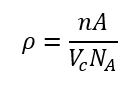
where n = number of atoms per unit cell, A = atomic weight, = unit cell volume, = Avogadro’s number.
Purpose – Relates atomic structure to macroscopic density of metals.
69. Polymorphism and Allotropy
Polymorphism – Ability of a material to exist in more than one crystal structure.
Allotropy – Polymorphism specifically for elemental solids (e.g., carbon as diamond, graphite).
Significance – Different structures have different physical properties (density, hardness, conductivity).
70. Crystal Systems
Seven crystal systems – Cubic, Tetragonal, Orthorhombic, Monoclinic, Triclinic, Hexagonal, Rhombohedral (Trigonal).
Classification based on – Unit cell edge lengths (a, b, c) and angles (α, β, γ).
Purpose – Helps identify symmetry and predict physical properties.
71. Crystallographic Points, Directions, And Planes
Points – Specific positions in the lattice, usually lattice points.
Directions – Vector connecting two points in the lattice; represented by [uvw].
Planes – Flat surfaces in the crystal; represented by (hkl) using Miller indices.
72. Point Coordinates
Lattice point coordinates – Fractional positions within a unit cell (0 ≤ x, y, z ≤ 1).
Used to – Define atomic positions for crystal structure calculations.
73. Crystallographic Directions
Direction vector [uvw] – Connects two lattice points; describes orientation in crystal.
Properties – Helps define anisotropic properties like slip directions in metals.
74. Crystallographic Planes
Miller indices (hkl) – Reciprocal of fractional intercepts of plane with axes.
Significance – Used to describe slip planes, cleavage planes, and density of atoms on surfaces.
75. Atomic Arrangements. Reduced-sphere FCC unit cell with (110) plane. Atomic Packing of an FCC (110) Plane
FCC (110) plane – Atoms arranged in close-packed rows.
Planar density – Fraction of area covered by atoms in that plane; highest in close-packed directions.
76. Atomic Arrangements. Reduced-sphere BCC unit cell with (110) plane. Atomic Packing of a BCC (110) Plane
BCC (110) plane – Atoms less densely packed than FCC.
Planar density – Lower than FCC (110); affects slip and deformation behavior.
77. Linear and Planar Densities. Linear density for FCC unit cell in the [110] direction
Linear density – Number of atoms per unit length along a crystallographic direction.
[110] FCC direction – Most densely packed; highest linear density.
78. Linear and Planar Densities. Planar density for FCC (110) plane
Planar density – Number of atoms per unit area of the plane.
FCC (110) plane – High planar density; important for slip and deformation.
79. Close-Packed Crystal Structures
Close-packed structures – FCC and HCP.
Properties – Maximum packing efficiency (APF = 0.74), high density, high coordination number (12).
80. Crystal Structure of Metals. Polymorphism and Allotropy
Metals – Can exhibit polymorphism at different temperatures/pressures (e.g., iron: BCC → FCC).
Allotropy – Different crystal forms of the same metal have different mechanical properties.
81. Crystal Structure of Ceramics
Ceramics – Usually ionic or covalent bonding; crystal structures determined by cation-anion size ratio.
Coordination – Number of nearest neighbor ions varies; affects density and mechanical properties.
82. Molecular Structure. Mer Structures of the More Common Polymeric Materials
PTFE – Fluorine substituted polymer.
PVC – Chlorine substituted polymer.
PP – Methyl (CH3) substituted polymer.
83. The Molecular Structure of Polymers. Types of Polymers by Observing the Repeating Unit
Homopolymer – All repeating units identical.
Copolymer – Two or more different repeating units.
Block copolymer – Different units arranged in blocks.
84. The Molecular Structure of Polymers. Types of Polymers by Observing the Way of Joining the Mer Units
Linear – Mer units end-to-end, spaghetti-like chains.
Branched – Side chains attached to main chain.
Cross-linked – Covalent bonds connect chains.
Network – 3D interconnected structure.
85. Crystalline and Noncrystalline Materials
Crystalline – Periodic, ordered arrangement of atoms.
Noncrystalline (amorphous) – No long-range order; structure resembles a frozen liquid.
86. Single Crystals
Single crystal – Perfect, uninterrupted periodic structure throughout the specimen.
Properties – Highly anisotropic; direction-dependent mechanical and physical properties.
87. Polycrystalline Materials
Polycrystalline – Aggregates of many small crystals (grains).
Grain boundaries – Regions of atomic mismatch between grains.
Properties – Often isotropic at macroscopic scale due to random grain orientation.
88. Anisotropy
Anisotropy – Direction-dependent properties in crystals.
Examples – Elastic modulus, electrical conductivity, refractive index vary with crystallographic direction.
Dependence – Increases with decreasing symmetry (triclinic > cubic).
89. Noncrystalline Solids
Amorphous solids – Lack long-range atomic order.
Examples – Glass, some polymers.
Properties – Isotropic; lower thermal conductivity than crystalline counterparts.
90. Imperfections in Solids. Range of Scales for the Various Classes of Defects
Defects – Deviations from perfect crystal lattice.
Scales – Point defects (atomic), linear defects (dislocations), planar defects (grain boundaries), volume defects (voids, cracks).
Significance – Defects influence mechanical, electrical, thermal, and optical properties.
91. Point Defects. Vacancies and Self-Interstitials
Vacancy – Missing atom at a lattice site.
Self-interstitial – Extra atom positioned in between lattice sites.
Effect – Increase diffusion, influence mechanical strength and electrical properties.
92. Impurities in Solids. Impurity Point Defects
Substitutional impurity – Foreign atom replaces host atom.
Interstitial impurity – Foreign atom occupies interstitial site.
Effect – Alters electrical conductivity, hardness, and lattice parameters.
93. Two Most Common Ways to Specify Composition
Weight percent – Mass fraction of element/compound.
Atomic percent – Mole fraction or ratio of atoms in a material.
94. Miscellaneous Imperfections
Defects include – Frenkel defects (cation vacancy + interstitial), Schottky defects (paired cation-anion vacancies).
Effect – Affect density, diffusion, electrical properties.
95. Dislocations–Linear Defects
Edge dislocation – Extra half-plane of atoms inserted in crystal.
Screw dislocation – Lattice planes form a helical ramp around a line.
Effect – Facilitate plastic deformation; key to strengthening mechanisms.
96. Interfacial Defects
Planar imperfections – Grain boundaries, phase boundaries, twin boundaries.
Effect – Influence diffusion, corrosion, mechanical strength.
97. Bulk or Volume Defects
Three-dimensional defects – Pores, cracks, inclusions.
Effect – Reduce strength, increase fracture susceptibility.
98. Atomic Vibrations
Atoms in solids – Vibrate about equilibrium positions.
Effect – Contribute to heat capacity, thermal conductivity, and thermal expansion.
99. Elastic Deformation
Reversible deformation – Material returns to original shape when load is removed.
Characterized by – Stress proportional to strain (Hooke’s law).
100. Mechanical Behaviour
Response of material to applied forces – Includes elasticity, plasticity, creep, fatigue, and fracture.
101. Stress, Strain, Stiffness, And Strength
Stress – Force per unit area (σ = F/A).
Strain – Deformation per unit length (ε = ΔL/L).
Stiffness – Resistance to deformation (modulus of elasticity, E).
Strength – Maximum stress material can withstand before failure.
102. Modes of Loading
Tensile – Pulling apart.
Compressive – Pushing together.
Shear – Sliding layers past one another.
Torsion – Twisting.
Bending – Combination of tension and compression.
103. Tension Tests
Determine – Stress-strain behavior, yield strength, ultimate tensile strength, ductility.
Specimen – Standardized rod or dog-bone shape.
104. Stress-strain Curves And Moduli
Elastic region – Linear stress-strain relationship; modulus of elasticity (E).
Plastic region – Permanent deformation occurs; yield point marks transition.
105. Stress-Strain Behaviour
Initial linear – Elastic deformation.
Beyond yield – Plastic deformation.
Ultimate tensile stress – Maximum stress before necking.
Fracture – Point of material failure.
106. Anelasticity
Time-dependent, reversible deformation – Material slowly returns to original shape after stress removal.
Occurs – Due to internal friction and delayed atomic rearrangements.
107. Poisson’s Ratio
Ratio of lateral strain to axial strain in elastic deformation:
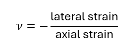
Typical metals – ν ≈ 0.3.
108. Yielding and Yield Strength
Yielding – Onset of plastic deformation.
Yield strength – Stress at which material begins to deform plastically.
109. Tensile Strength
Maximum stress material can withstand before necking occurs.
Also called – Ultimate tensile strength (UTS).
110. Ductility
Ability of a material to undergo plastic deformation before fracture.
Measured – % elongation or % reduction in area during tensile test.
111. Typical Mechanical Properties of Several Metals and Alloys
Example values – Steel: high strength and moderate ductility, Aluminum: low strength, high ductility.
Properties vary – With alloying, processing, heat treatment.
112. Modulus of Resilience
Energy per unit volume a material can absorb without permanent deformation:
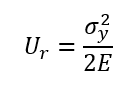
Where σ_y = yield stress, E = Young’s modulus.
113. Toughness
Energy per unit volume a material can absorb before fracturing.
Area under full stress-strain curve – Represents toughness.
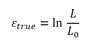
114. True Stress and Strain
True stress – Instantaneous load divided by instantaneous cross-sectional area.
True strain – Natural logarithm of ratio of current to original length:
115. Elastic Recovery After Plastic Deformation
Elastic Recovery After Plastic Deformation - After a material is loaded beyond its elastic limit, only the elastic portion of the deformation is recovered after unloading; plastic strain remains permanently. Important in springs, clips, and precision mechanical parts.
After unloading – Material partially recovers elastic strain; plastic strain remains.
Elastic recovery – Important in spring and precision components.
116. Hardness: Testing Methods and Scales
Hardness – Resistance to localized plastic deformation or indentation.
Hardness: Testing Methods and Scales - Hardness is the resistance of a material to localized plastic deformation or indentation. Testing methods include Brinell (steel/metal ball), Rockwell (conical/spherical indenter), Vickers (diamond pyramid indenter), and Mohs scale (scratch resistance). Hardness relates to wear resistance and strength.
Testing – Brinell, Rockwell, Vickers, Mohs scale.
117. The Origins of Strength
Strength arises from – Resistance to dislocation motion.
Factors – Crystal structure, defects, grain size, alloying.
The Origins of Strength - Strength arises from resistance to dislocation motion. Factors affecting strength include crystal structure (FCC vs BCC), defects, grain size (smaller grains increase strength), and alloying (solute atoms distort lattice to resist dislocations).
118. Manipulating Strength. Strengthening Metals
Methods – Work hardening, solid-solution strengthening, precipitation hardening, grain boundary strengthening.
Manipulating Strength. Strengthening Metals - Methods to strengthen metals include work hardening (increasing dislocation density), solid-solution strengthening (solute atoms distort lattice), precipitation hardening (small particles block dislocations), and grain boundary strengthening (smaller grains impede dislocation motion).
119. Mechanisms of Strengthening Metals
Work (strain) hardening – Increase dislocation density to impede motion.
Solid-solution strengthening – Solute atoms distort lattice and hinder dislocations.
Precipitation hardening – Small particles block dislocation movement.
Grain boundary strengthening – Reduce grain size to impede dislocation motion.
Mechanisms of Strengthening Metals - Work (strain) hardening increases dislocation density, making motion harder. Solid-solution strengthening uses solute atoms to distort the lattice. Precipitation hardening introduces particles that block dislocations. Grain boundary strengthening reduces grain size to block dislocation motion.
120. Grain Boundary Hardening
Smaller grains → more boundaries → dislocations blocked → higher strength.
Grain Boundary Hardening - Smaller grains create more grain boundaries, which block dislocation movement, increasing strength.
121. Solid-Solution Strengthening
Adding solute atoms → lattice distortion → dislocation motion harder → stronger metal.
Solid-Solution Strengthening - Adding solute atoms into a metal’s lattice causes distortion, which makes dislocation motion more difficult and increases the metal’s strength.
122. Strain Hardening
Plastic deformation → increased dislocation density → material harder and stronger.
Strain Hardening - Plastic deformation increases dislocation density in the metal, making further deformation harder and increasing both hardness and strength.
123. Strength and Ductility of Alloys
Alloy design – Balance strength and ductility for application.
Trade-off – Higher strength often reduces ductility; microstructure control can optimize both.
Strength and Ductility of Alloys - Alloy design balances strength and ductility for specific applications. Increasing strength often reduces ductility, but careful control of microstructure (grain size, phase distribution, and alloying) can optimize both properties.