AP Calculus AB Unit 1 Study Guide: Limits Involving Infinity (Asymptotes) + Intermediate Value Theorem
Infinite Limits and Vertical Asymptotes
What an infinite limit means
An infinite limit describes a function whose values grow without bound (positively or negatively) as the input approaches some finite number. In other words, the function does not approach a finite height near that input value: it “blows up.”
You write this using limit notation like:
This statement does not mean the limit equals a real number called infinity. Instead, it means that as x gets closer and closer to a (from both sides), the values of the function get arbitrarily large and positive. Similarly,
means the function values decrease without bound (becoming arbitrarily large in magnitude but negative).
A subtle but important vocabulary point: technically, an infinite limit means the (finite) limit does not exist (DNE), because it does not approach a real number. We still use the %%LATEX2%% and %%LATEX3%% notation to communicate how it fails to exist (the direction of the unbounded behavior).
A key idea is that infinite limits often come from expressions where a denominator approaches zero while the numerator stays nonzero, because dividing by a very tiny number creates outputs with very large magnitude.
Why infinite limits matter
Infinite limits are your formal tool for describing vertical blow-up behavior. They help you identify and justify vertical asymptotes, understand behavior near discontinuities, and communicate graph behavior near problem points precisely (especially for rational functions). They also connect directly to continuity: if the limit as x approaches a is infinite, then the limit at a does not exist as a finite number, so the function cannot be continuous at a.
One-sided infinite limits
Often the behavior differs depending on which side you approach from, so one-sided limits are essential.
means the function grows without bound as x approaches a from the left, and
means it decreases without bound as x approaches a from the right.
If the left-hand and right-hand behaviors are different, then there is no single two-sided statement like “the limit equals ” (even though you can still correctly state each one-sided limit).
Vertical asymptotes: what they are and how they relate
A vertical asymptote is a vertical line where the graph approaches that line as x gets close to a value, while the function values become unbounded.
In AP Calculus AB, the key connection is:
- If at least one one-sided limit is infinite, then there is a vertical asymptote.
More formally, is a vertical asymptote if
or
Be careful: a function can be undefined at a without having a vertical asymptote (for example, a removable discontinuity where the limit is finite).
How to find infinite limits (especially for rational functions)
Many infinite-limit questions involve rational functions:
where %%LATEX11%% and %%LATEX12%% are polynomials.
A reliable process near a suspected vertical asymptote is:
- Factor numerator and denominator.
- Check for cancellation.
- If a factor cancels, you may have a hole (removable discontinuity) instead of a vertical asymptote.
- For the remaining denominator, find where it equals zero. Those points are candidates for vertical asymptotes.
- To determine whether the function goes to %%LATEX14%% or %%LATEX15%% on each side, do a sign analysis near .
The “Non-Zero over Zero” rule (quick VA check)
For a rational function
a vertical asymptote occurs at if:
If both numerator and denominator are zero at the same x-value (the indeterminate form
), there is likely a removable discontinuity (a hole) after simplification, not a vertical asymptote.
Determining the direction (sign analysis)
Near %%LATEX22%%, if the denominator is close to %%LATEX23%% but positive, then the sign of the fraction matches the sign of the numerator; if the denominator is close to but negative, the sign flips. You can do this systematically by checking signs of factors, or you can “test” a value very close to the asymptote on the desired side.
Example (test-value sign analysis): Determine the behavior of
as x approaches 2 from the left.
At %%LATEX26%%, the numerator is positive and the denominator is zero, so there is a vertical asymptote at %%LATEX27%%. Choose a nearby point from the left, such as . Then the numerator is positive and the denominator is negative, so the fraction is negative and very large in magnitude. Therefore,
Notation reference (common limit statements)
| Meaning | Notation |
|---|---|
| Two-sided infinite limit (grows without bound) | |
| Two-sided infinite limit (decreases without bound) | |
| Left-hand infinite limit | |
| Right-hand infinite limit |
Worked Example 1: a “same on both sides” vertical blow-up
Consider:
The denominator is zero at %%LATEX35%%, so %%LATEX36%% is a candidate. The squared term is always positive (except it is zero at ). As x approaches 2, the denominator becomes a very small positive number, so the function becomes very large positive. Thus,
So is a vertical asymptote, and the graph shoots upward on both sides.
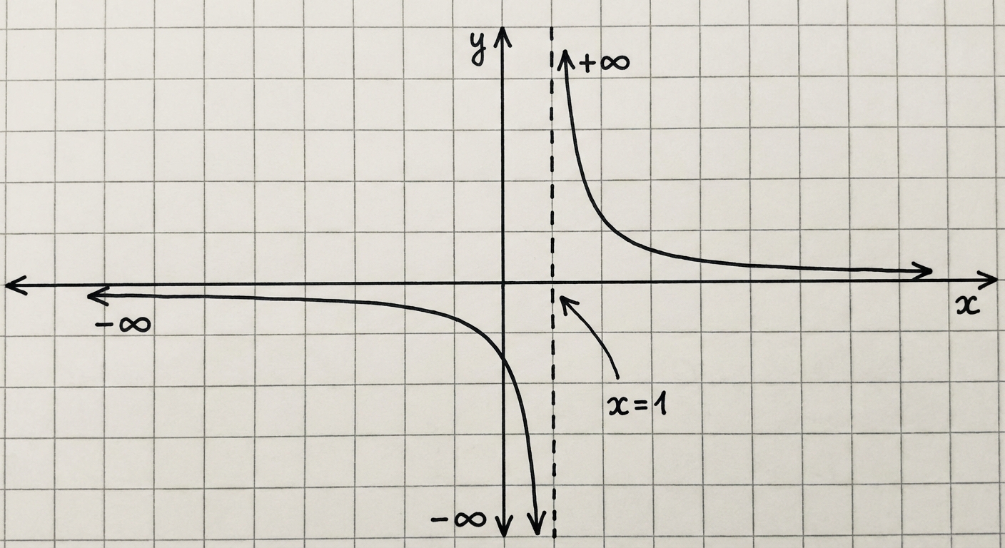
Worked Example 2: different one-sided behavior and a removable discontinuity
Let:
Factor the denominator:
So
For , you can cancel to get
This tells you two important things: (1) at %%LATEX45%% the original function is undefined but the limit may be finite (a hole), and (2) at %%LATEX46%% the denominator remains zero, indicating a vertical asymptote.
Using the simplified form for behavior near :
- As x approaches 1 from the left, is a small negative number, so the function is large negative.
- As x approaches 1 from the right, is a small positive number, so the function is large positive.
For , the limit is finite:
So is not a vertical asymptote; it is a removable discontinuity (a hole).
Exam Focus
Typical question patterns include finding one-sided infinite limits and stating whether a vertical asymptote exists, describing blow-up behavior from a graph or table using correct notation, and deciding whether a discontinuity is removable (hole) or infinite (vertical asymptote).
Common mistakes include treating like a number you can plug in, canceling factors but forgetting that cancellation creates a hole in the original function, and assuming the behavior is the same from both sides without checking signs (especially with odd powers like
). Also avoid the trap of claiming “vertical asymptotes are just zeros of the denominator”: if the simplified form cancels the problematic factor (creating
before simplifying), you have a hole, not a vertical asymptote.
Limits at Infinity and Horizontal Asymptotes
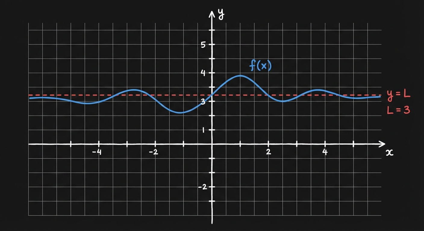
What a limit at infinity means
A limit at infinity describes what happens to a function as x becomes very large (to the right) or very negative (to the left). Instead of zooming in near a point, you’re looking at the graph’s long-run behavior.
means as x increases without bound, the function gets closer and closer to L. Similarly,
means as x decreases without bound, the function approaches L.
Horizontal asymptotes: what they tell you
A horizontal asymptote is a horizontal line that the function approaches as x goes to infinity and/or negative infinity. The connection is direct:
- If
then is a horizontal asymptote to the right.
- If
then is a horizontal asymptote to the left.
A common misconception is that a function can never cross a horizontal asymptote. It can cross; the asymptote describes end behavior, not a barrier.
Why limits at infinity matter
Limits at infinity help you sketch rational functions, interpret models where a quantity levels off over time, and recognize asymptotes as long-term trends even when short-term behavior is complicated.
How to compute limits at infinity for rational functions (degree comparison)
For many AP Calculus AB problems,
where %%LATEX65%% and %%LATEX66%% are polynomials. The key tool is comparing degrees (highest powers).
Case 1: Degree of numerator < degree of denominator (bottom heavy)
The denominator grows faster, so the fraction goes to zero:
and similarly for %%LATEX68%%. The horizontal asymptote is %%LATEX69%%.
Case 2: Degrees equal (balanced)
The limit approaches the ratio of leading coefficients. If
and
then
The same usually holds for when degrees match, because leading terms dominate.
Case 3: Degree of numerator > degree of denominator (top heavy)
The function does not approach a finite constant, so there is no horizontal asymptote. In many such cases the limit is %%LATEX74%% or %%LATEX75%% (check signs of leading terms). If the numerator’s degree is exactly one higher than the denominator’s, the end behavior is often governed by a slant (oblique) asymptote.
Memory aid: BOBO BOTN EATS DC
This mnemonic summarizes the rational-function degree cases.
- BOBO: Bigger On Bottom, Zero
- BOTN: Bigger On Top, None (often infinity behavior)
- EATS DC: Exponents Are The Same, Divide Coefficients
A “divide by highest power” method (mechanism)
A practical way to compute these limits is to divide numerator and denominator by the highest power of x appearing in the denominator (or by the highest power overall). This rewrites the function so that terms like
and
clearly go to zero as x goes to infinity or negative infinity.
For example:
and you use
and
Worked Example 1: equal degrees (ratio of leading coefficients)
Compute:
Divide top and bottom by :
As x approaches infinity, the fractional pieces go to zero, so
So is a horizontal asymptote to the right. In this example it is also the horizontal asymptote to the left:
Worked Example 2: smaller numerator degree (approaches zero)
Compute:
Here the denominator degree is larger, so the limit should be zero. Dividing by confirms:
So
Thus is a horizontal asymptote.
Subtle point: right-end vs left-end behavior can differ
Some functions approach different values as x approaches infinity versus negative infinity, so it is good practice to check both directions unless the function’s structure clearly makes them the same.
Limits at infinity for non-rational functions (dominance and bounding)
Do not rely solely on polynomial degree rules when the function is not purely rational. Instead, identify which term dominates (grows fastest in magnitude).
A common hierarchy of dominance from fastest growth to slowest growth is:
- Exponentials (like %%LATEX92%% and %%LATEX93%%)
- Polynomials (like %%LATEX94%% and %%LATEX95%%)
- Logarithms (like )
- Bounded functions (like %%LATEX97%% and %%LATEX98%%)
Example (exponential dominates polynomial):
because the exponential grows much faster than the polynomial.
Important note on oscillating (bounded) functions: Since
the numerator in
is bounded while the denominator grows without bound, so
Radical sign errors (a common trap at negative infinity)
When radicals involve squares, remember the absolute value identity:
So for
as x approaches negative infinity, , so the expression behaves like
and the limit is
not .
Exam Focus
Typical question patterns include finding
and interpreting the horizontal asymptote, determining horizontal asymptotes of rational functions using degrees or algebraic manipulation, and reading end behavior from a graph (both right and left ends).
Common mistakes include mixing up vertical and horizontal asymptotes (vertical involves x approaching a finite number; horizontal involves x approaching infinity or negative infinity), dividing by the wrong power of x or forgetting to divide every term, and assuming a horizontal asymptote can never be crossed. Also watch two classic pitfalls: confusing the line types (horizontal asymptotes are %%LATEX110%%, not %%LATEX111%%), and mishandling radicals at negative infinity by forgetting
Intermediate Value Theorem (IVT)
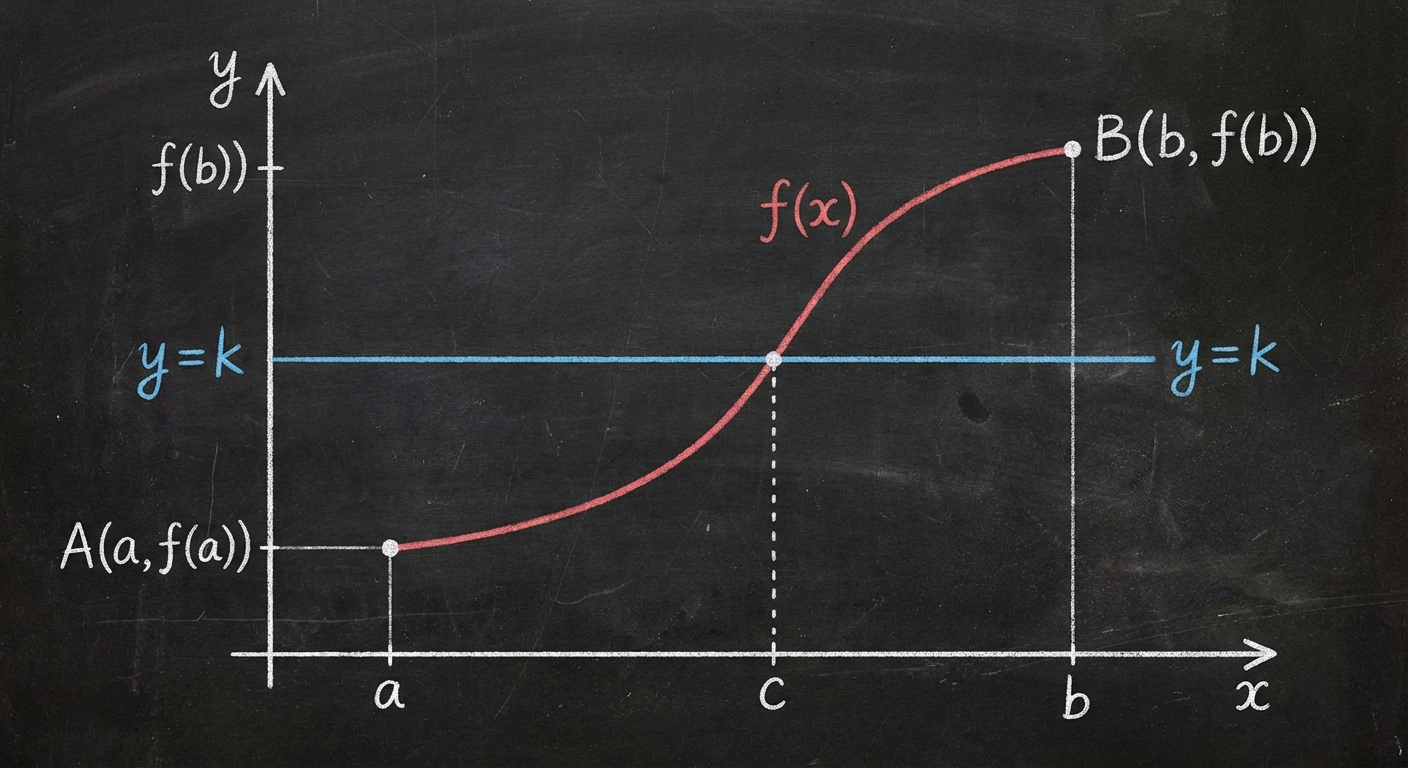
What the Intermediate Value Theorem says
The Intermediate Value Theorem (IVT) is a fundamental result about continuous functions. It formalizes the idea that a continuous function cannot “jump over” values.
If a function is continuous on a closed interval and you choose any target value between its endpoint outputs, the function must hit that target somewhere in the interval.
A precise statement is: if %%LATEX113%% is continuous on %%LATEX114%% and %%LATEX115%% is any number between %%LATEX116%% and %%LATEX117%%, then there exists at least one number %%LATEX118%% in such that
Many AP-style “existence” conclusions are written with %%LATEX121%% in the open interval %%LATEX122%%. That happens when the target value is strictly between the endpoint values. If the target value equals an endpoint value, the theorem can be satisfied by choosing %%LATEX123%% or %%LATEX124%%.
A particularly important special case is when %%LATEX125%%. If %%LATEX126%% and have opposite signs, then the function must cross the x-axis somewhere between them, so there is at least one root.
Why IVT matters in a unit about limits and continuity
IVT is one of the first big payoffs of continuity. Limits and continuity are not just about computing numbers; they let you make guarantees.
IVT is used to prove an equation has a solution without actually finding it, justify that a function must attain certain values on an interval, and support numerical methods like bisection that approximate solutions by narrowing an interval where a root must exist.
It also clarifies what discontinuities break: if a function is not continuous on (for example, it has a vertical asymptote inside the interval), then IVT may fail because the function can “skip” values.
Conditions for use (the hypothesis you must state)
On AP Free Response, points are often earned by explicitly verifying the hypotheses. A strong IVT setup checks:
- Continuity on the entire interval .
- The target value is between the endpoint outputs. Many textbook summaries also include %%LATEX130%% and “strictly between” language; that’s the common root-finding case where you want to guarantee a solution in %%LATEX131%%.
If either continuity or the “between” condition fails, you cannot conclude existence of .
How to use IVT on AP-style problems (step-by-step)
Most IVT problems follow a predictable structure.
- Define a function whose root or target value corresponds to the statement you want.
- For solving , define
and look for .
Check continuity of the function on .
- Polynomials are continuous everywhere.
- Rational functions are continuous where their denominators are nonzero.
- Trig functions like sine and cosine are continuous everywhere.
Evaluate endpoint values.
Confirm the “between” condition (often a sign change for root problems).
State the conclusion clearly: there exists at least one %%LATEX137%% in the interval such that %%LATEX138%% equals the target value.
Worked Example 1: guaranteeing a root
Show that the equation
has a solution between 1 and 2.
Let
This is a polynomial, so it is continuous on . Compute endpoints:
Since 0 is between -1 and 5, IVT guarantees there exists at least one %%LATEX144%% in %%LATEX145%% such that
IVT does not give the exact value of , and it does not guarantee the solution is unique.
Worked Example 2: proving two functions intersect
Show that %%LATEX148%% and x intersect somewhere in %%LATEX149%%.
An intersection means
Define
Both %%LATEX152%% and x are continuous everywhere, so %%LATEX153%% is continuous on . Evaluate endpoints:
Since %%LATEX157%%, this endpoint value is negative. Because %%LATEX158%% is positive and %%LATEX159%% is negative, IVT guarantees there exists at least one %%LATEX160%% in such that
which means
Example writing sample for the AP Exam
A common FRQ expectation is a clear, sentence-style justification. For example:
“Since %%LATEX164%% is continuous on %%LATEX165%%, and %%LATEX166%% and %%LATEX167%%, by the Intermediate Value Theorem there must exist a value %%LATEX168%% in %%LATEX169%% such that .”
What goes wrong: when you cannot use IVT
IVT fails if the function is not continuous on the entire interval. A classic trap is a rational function with a vertical asymptote inside the interval.
For instance,
on %%LATEX172%% is not continuous because it is undefined at %%LATEX173%%. Even if
and
you cannot conclude there exists with
In fact, this function is never zero. This is a direct connection back to limits involving infinity: a vertical asymptote often signals discontinuity that breaks IVT assumptions.
Exam Focus
Typical question patterns include using IVT to show a solution exists to
on an interval, showing two graphs intersect by applying IVT to a difference function, and explaining why IVT cannot be applied on a given interval by identifying a discontinuity.
Common mistakes include forgetting to justify continuity on (especially for rational functions), thinking IVT finds the solution (it only proves existence), and claiming uniqueness when IVT only guarantees at least one solution. A frequent scoring pitfall on FRQs is applying IVT without explicitly stating continuity; writing the continuity justification is often worth a point.