Comprehensive Guide to Unit 4: Vectors, Matrices, and Linear Transformations

Fundamentals of Plane Vectors

Vectors in Two Dimensions

A vector is a mathematical object that possesses both magnitude (length) and direction. In AP Precalculus, we primarily analyze vectors in a two-dimensional plane.

Vector Notation and Components

Vectors are often represented by directed line segments (arrows) or algebraic pairs.

• Standard Form: $\vec{v} = \langle a, b \rangle$
  • $a$ is the horizontal component.
  • $b$ is the vertical component.
• Unit Basis Vectors: $\vec{v} = a\mathbf{i} + b\mathbf{j}$, where $\mathbf{i} = \langle 1, 0 \rangle$ and $\mathbf{j} = \langle 0, 1 \rangle$.

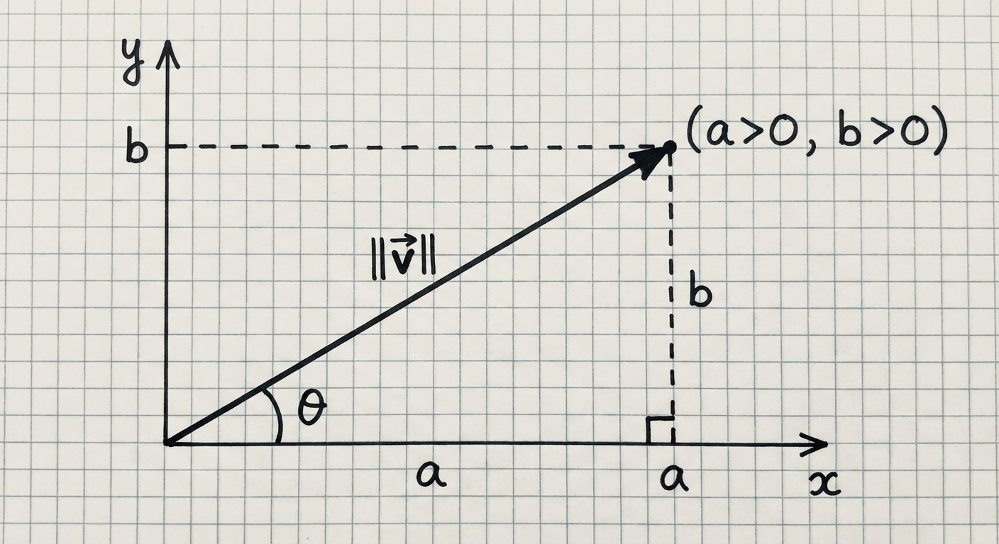
Magnitude and Direction

Given a vector $\vec{v} = \langle a, b \rangle$:

1. Magnitude (Length): Calculated using the Pythagorean theorem.
   $||\vec{v}|| = \sqrt{a^2 + b^2}$
2. Direction Angle ($\theta$): The angle the vector makes with the positive x-axis. $\tan(\theta) = \frac{b}{a}$
   • Note: You must adjust $\theta$ based on the quadrant where $(a,b)$ lies.

Vector Arithmetic

We can perform arithmetic operations on vectors component-wise.

• Vector Addition: $\vec{u} + \vec{v} = \langle u<em>1 + v</em>1, u<em>2 + v</em>2 \rangle$
  • Geometrically: This follows the head-to-tail method (triangle rule) or parallelogram rule.
• Scalar Multiplication: $k\vec{v} = \langle ka, kb \rangle$
  • Scales the length by $|k|$.
  • If $k < 0$, the direction reverses.

Vector-Valued Functions

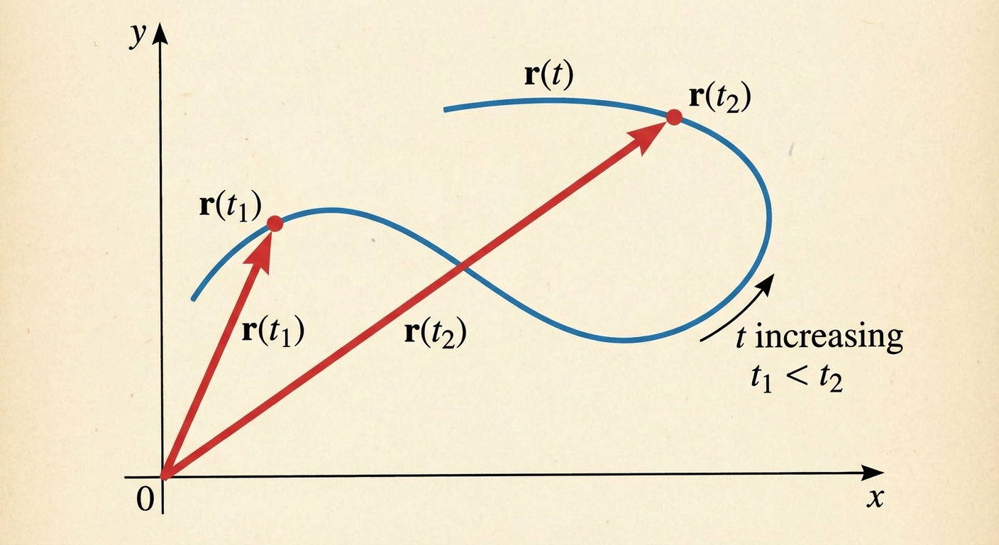
A vector-valued function takes a scalar input (typically time, $t$) and outputs a vector.

$\vec{r}(t) = \langle f(t), g(t) \rangle$

Motion Along a Curve

This concept ties directly to parametric equations. While parametric equations describe $x$ and $y$ separately, a vector-valued function describes the position vector pointing from the origin to the point $(x(t), y(t))$ on the curve.

• Input domain: The set of allowed $t$ values.
• Output range: Variations of the position vector $\vec{r}(t)$.

Example:
If $\vec{r}(t) = \langle t^2, 2t \rangle$ for $t \ge 0$:

• At $t=1$, position is $\langle 1, 2 \rangle$.
• At $t=2$, position is $\langle 4, 4 \rangle$.

Matrices and Matrix Operations

A matrix is a rectangular array of numbers arranged in rows and columns. A matrix with $m$ rows and $n$ columns has dimensions $m \times n$.

Basic Operations

1. Addition/Subtraction: Only possible if dimensions represent the exact same size. Add corresponding entries.
2. Scalar Multiplication: Multiply every entry in the matrix by the scalar constant $k$.

Matrix Multiplication

This is a non-commutative operation (order matters).

• Condition: To multiply Matrix $A$ ($m \times n$) by Matrix $B$ ($n \times p$), the number of columns in $A$ must equal the number of rows in $B$.
• Result: The resulting matrix will have dimensions $m \times p$.

$\text{If } A = \begin{bmatrix} a & b \ c & d \end{bmatrix} \text{ and } B = \begin{bmatrix} x \ y \end{bmatrix}, \text{ then } AB = \begin{bmatrix} ax + by \ cx + dy \end{bmatrix}$

To find the entry in row $i$ and column $j$ of the product, find the dot product of row $i$ from the first matrix and column $j$ from the second matrix.

Linear Transformations and Matrices

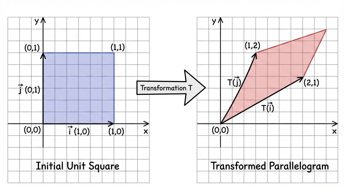
Matrices can be viewed as functions that map (transform) vectors from one position to another. The input is a vector $\vec{x}$, and the function is the matrix multiplication $T(\vec{x}) = A\vec{x}$.

Geometric Interpretation on the Plane

For a $2 \times 2$ matrix transforming a $2 \times 1$ vector:

• The Identity Matrix ($I$): $\begin{bmatrix} 1 & 0 \ 0 & 1 \end{bmatrix}$ leaves a vector unchanged.
• Zero Matrix: Maps all vectors to $\langle 0, 0 \rangle$.
• Dilation: $\begin{bmatrix} k & 0 \ 0 & k \end{bmatrix}$ scales the vector by factor $k$.
• Reflection (over x-axis): $\begin{bmatrix} 1 & 0 \ 0 & -1 \end{bmatrix}$ flips the y-coordinate.
• Rotation (90° CCW): $\begin{bmatrix} 0 & -1 \ 1 & 0 \end{bmatrix}$ maps $\langle 1, 0 \rangle \to \langle 0, 1 \rangle$ and $\langle 0, 1 \rangle \to \langle -1, 0 \rangle$.

Matrices as Functions

Just as we analyze functions for inverses and domain, we analyze matrices similarly.

The Determinant

For a $2 \times 2$ matrix $A = \begin{bmatrix} a & b \ c & d \end{bmatrix}$, the determinant is:

$\det(A) = ad - bc$

Significance of the Determinant:

1. Area Scale Factor: The absolute value $|\det(A)|$ represents the factor by which the matrix scales the area of a region. If $\det(A) = 2$, shapes become twice as large after transformation.
2. Invertibility: If $\det(A) = 0$, the matrix squashes the plane into a line or a point (loss of dimension). Such a matrix has no inverse (it is singular).

The Inverse Matrix

The inverse matrix $A^{-1}$ "undoes" the transformation of $A$. It exists only if $\det(A) \neq 0$.

$A^{-1} = \frac{1}{ad-bc} \begin{bmatrix} d & -b \ -c & a \end{bmatrix}$

Property: $A \cdot A^{-1} = I$ (The Identity Matrix).

If we view a matrix as a function $f(\vec{v}) = A\vec{v}$, then the inverse function is $f^{-1}(\vec{v}) = A^{-1}\vec{v}$.

Common Mistakes & Pitfalls

1. Matrix Multiplication Order: Students often think $AB = BA$. This is false for matrices. Always maintain strict left-to-right order.
2. Determinant Denominator: When calculating the inverse, remember to divide by the determinant ($ad-bc$). If you multiply by it, your result is wrong.
3. Vector Direction (Quadrants): When finding $\theta = \tan^{-1}(b/a)$, the calculator gives the reference angle. You must visualize the point $(a,b)$ to determine the correct quadrant (e.g., adding $180^\circ$ or $\pi$ if vectors are in Q2/Q3).
4. Dimension Mismatch: Attempting to multiply a $2 \times 2$ matrix by a $1 \times 2$ (row) vector instead of a $2 \times 1$ (column) vector. The inner dimensions must match.