Wk 6: Multi-Factor Between-Participant Designs - Regression

Correlation, Z-Scores, and Variance Explained

• Correlation and variance explained are two variables that are fundamentally linked; stronger correlations imply that more variance is explained in the criterion.

• This connection allows for the estimation of $F$ statistics in regression without solving for regression coefficients, predicting data, or manually summing squared residuals. Instead, sets of correlation coefficients can be used to calculate $R_{reg}^2$.

• Correlation is a standardized measure of the degree of association between two variables, which can be calculated in two ways:

  • Calculating the covariance first and then standardizing.

  • Standardizing the variables into Z-scores first and then calculating the covariance.

• Standardization before calculating covariance is often easier. If systematic variance exceeds unsystematic variance, the vector will correlate with the criterion.

• This means positive Z-scores on the vector will correspond with positive Z-scores on the criterion, and negative Z-scores will correspond similarly.

• The average product of Z-scores results in the correlation coefficient ($r$).

Multi-Factor Between-Participant Designs

• A multi-factor design involves the manipulation of more than one independent variable (IV) or factor.

  • e.g. medication x2, and therapy type x2

• It is termed a factorial design if all possible conditions created by crossing the factors are included in the study.

• In a factorial design, researchers examine two types of effects:

  • Main Effect: The effect of one factor considered separately from the effect of the other factor.

  • Interaction: The effect of one factor in combination with another factor. This occurs when the effect of Factor A differs across different levels of Factor B (and vice versa).

• Example of a 2-factor design:

  • Main effect of Factor A (averaged across levels of Factor B).

  • Main effect of Factor B (averaged across levels of Factor A).

  • An interaction effect ($A \times B$).

Factorial Designs in Regression and Vector Coding

• Estimating main effects and interactions in regression follows the same process as one-way designs: coding vectors to capture between-groups variability.

• Vector Counts:

  • In one-way designs, there is one set of vectors containing one less vector than the number of conditions.

  • In factorial designs, sets of vectors are created for each main effect and each interaction.

  • In a $2 \times 2$ design, there is 1 vector for the first factor, 1 vector for the second factor, and 1 vector for the interaction.

• Coding Schemes:

  • Dummy-coding: Participants in one condition are coded as $1$ and others as $0$.

  • Contrast-coding: Participants in one condition are coded as $1$ and others as $-1$.

• 3-Level Factors: These require two vectors ($V1$ and $V2$) to capture the variability among three groups.

• Coding the Interaction:

  • Interaction vectors are created by multiplying the vectors coding for the main effects.

  • For a $2 \times 2$ design with $V1$ (Factor A) and $V2$ (Factor D), the interaction vector ($V3$) is calculated as $V1 \times V2$.

  • For a $3 \times 2$ design with Factor A ($V1$, $V2$) and Factor D ($V3$), there are two interaction vectors: $V4 = V1 \times V3$ and $V5 = V2 \times V3$.

Regression Equations for Factorial Designs

• The linear regression equation adds terms for every coded vector.

• $2 \times 2$ Design Equation:

  • $\hat{Y} = a + b_1X_1 + b_2X_2 + b_3X_1X_2$

  • $b_1$ is the slope for Factor A; $b_2$ is the slope for Factor D; $b_3$ is the slope for the interaction.

• $3 \times 2$ Design Equation:

  • $\hat{Y} = a + b_1X_1 + b_2X_2 + b_3X_3 + b_4X_1X_3 + b_5X_2X_3$

  • $b_1$ and $b_2$ represent the slopes for the two vectors of Factor A; $b_3$ represents Factor D; $b_4$ and $b_5$ represent the interaction vectors.

• Interpretation of Intercept ($a$) and Slopes ($b$):

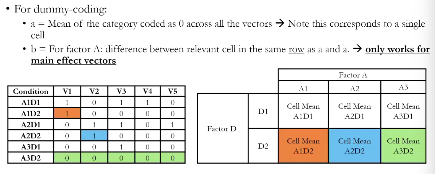
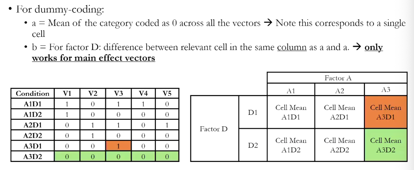
  • Dummy-coding: $a$ is the mean of the category coded as $0$ across all vectors (a single cell). $b$ for a main effect vector is the difference between the relevant cell in the same row/column as $a$ and the value of $a$.

  

  • Contrast-coding:

    • $a$ is the grand mean.

    • $b$ = difference between mean of category coded 1 on that vector and grand mean

• 

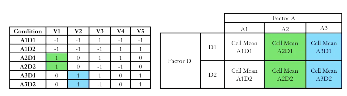
  green: A2 marginal mean vs grand mean

    blue: A3 marginal mean vs grand mean

Vector Sets and Calculating $R_{Reg}^2$

• To derive $F$ values for each effect (Main Effect A, Main Effect D, Interaction AXD), separate $R_{Reg}^2$ values must be calculated: $R_A^2$, $R_D^2$, and $R_{AxD}^2$.

  • variance explained by the whole model

  • variance explained by factor A

  • variance explained by factor D

  • variance explained by interaction

• 

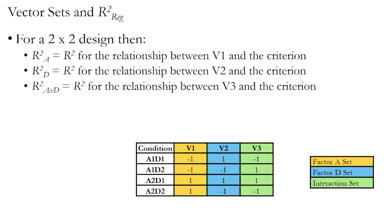
• If a set contains only a single vector, $R_{Reg}^2$ is simply the square of the correlation between that vector and the criterion ($r^2$).

• If a set contains more than one vector (e.g., Factor A in a $3 \times 2$ design), the inter-correlation between those vectors must be controlled using the formula:

  • $R_{Reg}^2 = \frac{r_1^2 + r_2^2 - (2 \times r_1 \times r_2 \times r_{12})}{1 - r_{12}^2}$

  • Where $r_1$ and $r_2$ are correlations with the criterion and $r_{12}$ is the correlation between the vectors in the set.

Inference and Significance Testing

• Residual Variance: $R_{Res}^2 = 1 - \sum R_{Reg}^2 = 1 - (R_A^2 + R_D^2 + R_{AxD}^2)$.

• Degrees of Freedom ($df$):

  • $df_A = k_A$ (number of vectors for Factor A).

  • $df_D = k_D$ (number of vectors for Factor D).

  • $df_{AxD} = k_A \times k_D$ (product of the degrees of freedom of the main factors).

  • $df_{Res} = N - \sum k - 1$.

• Mean Squares ($MS$):

  • $MS_A = R_A^2 / df_A$

  • $MS_D = R_D^2 / df_D$

  • $MS_{AxD} = R_{AxD}^2 / df_{AxD}$

  • $MS_{Res} = R_{Res}^2 / df_{Res}$

• F-Ratios:

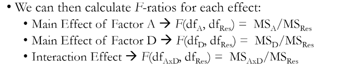
  • $F(df_{Effect}, df_{Res}) = MS_{Effect} / MS_{Res}$.

  • If F_{obs} > F_{crit}, reject the null hypothesis ($H_0$).

Example 1: $2 \times 2$ Factorial Design

• Design: 2 (Animal Type: Approach/Avoid) $\times$ 2 (Mood: Positive/Negative) Between-Participants.

• Animal Groups:

  • Approach: dog, cat, rabbit, beaver, quokka.

  • Avoid: lion, tiger, bear, rhino, bison.

• Dependent Variable (DV): Number of animals remembered from a list.

• Data Recap:

  • Grand mean ($a$) = $6.04$.

  • $b_1$ (Approach mean - Grand mean) = $4.92 - 6.04 = -1.12$.

  • $b_2$ (Positive mean - Grand mean) = $5 - 6.04 = -1.04$.

• Step-by-Step Results:

  • Correlation ($r$) with criterion: $V1 = -0.566$, $V2 = -0.524$, $V3 = 0.314$.

  • $R_{AnimalType}^2 = 0.32$, $R_{Mood}^2 = 0.27$, $R_{Int}^2 = 0.10$.

  • $R_{Res}^2 = 1 - (0.32 + 0.27 + 0.10) = 0.307$.

  • Degrees of freedom: $df_{AnimalType} = 1$, $df_{Mood} = 1$, $df_{Int} = 1$, $df_{Res} = 20$.

  • Mean Squares: $MS_{AnimalType} = 0.32$, $MS_{Mood} = 0.27$, $MS_{Int} = 0.10$, $MS_{Res} = 0.015$.

  • F-ratios:

    • Animal Type: $F(1, 20) = 0.32 / 0.015 = 20.83$ (p < 0.001).

    • Mood: $F(1, 20) = 0.27 / 0.015 = 17.86$ (p < 0.001).

    • Interaction: $F(1, 20) = 0.10 / 0.015 = 6.43$ (p < 0.001).

• Interpretation: Significant main effects (greater memory for avoid animals and negative moods) and a significant interaction.

Example 2: $3 \times 2$ Factorial Design

• Design: 3 (Animal Type: Approach/Avoid/Neutral) $\times$ 2 (Mood: Positive/Negative).

• Contrast Coding Scheme:

  • V1 (Avoid vs. Others): Avoid = $1$, Approach = $-1$, Neutral = $0$.

  • V2 (Neutral vs. Others): Neutral = $1$, Approach = $-1$, Avoid = $0$.

  • V3 (Mood): Positive = $1$, Negative = $-1$.

• Calculations:

  • Grand Mean ($a$) = $5.64$.

  • $b_1$ (Avoid Mean - Grand Mean) = $7.17 - 5.64 = 1.53$.

  • $b_2$ (Neutral Mean - Grand Mean) = $4.83 - 5.64 = -0.81$.

  • $b_3$ (Positive Mean - Grand Mean) = $4.28 - 5.64 = -1.36$.

• Correlations and $R^2$:

  • Animal Type Set ($V1, V2$): $r_1 = 0.420$, $r_2 = -0.016$, $r_{12} = 0.50$. $R_{AnimalType}^2 = 0.244$.

  • Mood Set ($V3$): $r = -0.622$. $R_{Mood}^2 = 0.39$.

  • Interaction Set ($V4, V5$): $r_4 = -0.233$, $r_5 = -0.295$, $r_{45} = 0.50$. $R_{Int}^2 = 0.097$.

• F-Statistics:

  • $R_{Res}^2 = 0.27$, $df_{Res} = 30$, $MS_{Res} = 0.009$.

  • Animal Type: $F(2, 30) = 0.12 / 0.009 = 13.47$ (p < 0.001).

  • Mood: $F(1, 30) = 0.39 / 0.009 = 42.72$ (p < 0.001).

  • Interaction: $F(2, 30) = 0.049 / 0.009 = 5.36$ (p < 0.001).

Effect Sizes

• While Significance testing ($p$-values) helps decide whether to reject $H_0$, effect sizes describe the magnitude.

• $R_{Reg}^2$: The proportion of total criterion variance explained by an effect. However, it does not account for the overlap or presence of other effects.

• Partial $R^2$: The proportion of residual criterion variance explained by an effect, controlling for other effects.

• Formula: $\text{Partial } R^2 = \frac{R_{Reg}^2}{R_{Res}^2 + R_{Reg}^2}$.

• Cut-offs for $R^2$ and Partial $R^2$:

  • Small: >0.01 to $0.06$.

  • Medium: >0.06 to $0.14$.

  • Large: >0.14.

• Comparison Example ($2 \times 2$):

  • Animal Type: $R^2 = 0.32$; Partial $R^2 = 0.32 / (0.307 + 0.32) = 0.51$.

  • Mood: $R^2 = 0.27$; Partial $R^2 = 0.27 / (0.307 + 0.27) = 0.47$.

  • Interaction: $R^2 = 0.10$; Partial $R^2 = 0.10 / (0.307 + 0.10) = 0.24$.