Equilibrium in the Goods Market

Learning Objectives for Unit 7: Equilibrium in the Goods Market

What Determines the Demand for Goods and Services?

• The demand for goods and services is addressed through

• the four components of Gross Domestic Product (GDP).

• The fundamental equation for output is:

  • $Y = C + I + G$

• Where:

  • $Y$ is Total Output (GDP).

  • $C$ is Consumption.

  • $I$ is Investment.

  • $G$ is Government Purchases.

Consumption ($C$)

• Definition of Consumption: Households receive income (Y) from their labor and their ownership of capital and they pay taxes (T) to the government. Income remaining after taxes is referred to as disposable income.

• Disposable Income Equation:

  • $\text{Disposable Income} = Y - T$

  • Where $Y$ is total income and $T$ is taxes.

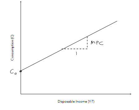
• The Consumption Function: Consumption decisions are made based on disposable income. The relationship is expressed as:

  • $C = C(Y - T)$

    The C Infront of the equation is us trying to find the total consumption. While the other C is the consumption function

• The Marginal Propensity to Consume (MPC): This is the amount by which consumption changes when disposable income increases by one dollar.

  • The change in consumption ($\Delta C$) is equal to the MPC multiplied by the change in income ($\Delta Y$).

  • $MPC = \frac{\Delta C}{\Delta Y}$

• Consumption Function Components: The function can be written as $C = C_0 + MPC(Y - T)$.

• $C_0$ represents Autonomous Consumption, which is the amount spent even if disposable income ($Y - T$) is zero.

• Aggregate Saving ($S$): Is the portion of aggregate income that is not consumed.

  • $S = (Y - T) - C$

• Marginal Propensity to Save (MPS): The fraction of a change in income that is saved.

  • $MPS = 1 - MPC$

  • Therefore, $MPC + MPS = 1$

• Other Factors Influencing Consumption:

  • Wealth.

  • The Interest Rate.

  • Expectations of the Future.

Investment ($I$)

• Definition:

• Investment goods are products used to help produce other goods or services in the future. They are also called capital goods.

• Both firms and households purchase investment goods.

• • These are things businesses buy to improve production, efficiency, or future profits, not for immediate personal use.

  • Examples: Firms buy investment goods to add to their stock of capital and to replace existing capital as it wears out.

  • Households buy new houses, which are categorized as part of investment.

• Scale of Investment: Total investment in the United States averages approximately $15\%$ of GDP.

• Role of the Interest Rate: The quantity of planned investment demand depends on the interest rate ($r$), which measures the cost of the funds used to finance investment.

  • For an investment to be profitable, the return must be greater than the interest rate.

  • Hypothetical Example: If an investment returns $10\%$ per year, this project is only profitable if the interest rate is less than $10\%$.

  • This makes sense if you have to borrow money in order to finance your investment. But what if you have enough cash to pay for your investment yourself (don’t have to pay interest)?

  • Because you are using your own cash to finance your investment you are

  • forgoing the interest payment that you would receive if you loaned that money out to someone else.

  • The interest rate in this case represents the opportunity cost of using your own cash to finance your investment

• Finance and Opportunity Cost:

  • If a firm borrows money, the interest rate is a direct cost.

  • If a firm uses its own cash, it doesn't pay interest. However, by using its own cash, it is forgoing the interest payment it would receive if it loaned that money out. Thus, the interest rate represents the opportunity cost of using internal funds.

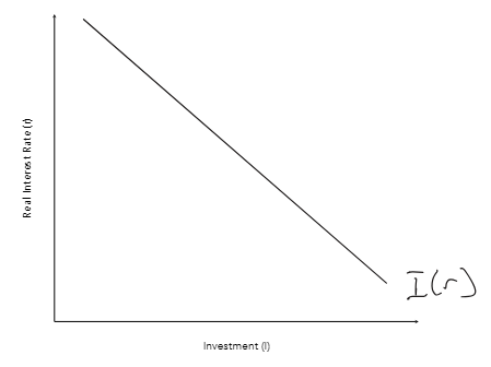
• Real Interest Rate vs. Investment: There is a negative relationship between the real interest rate and Gross Domestic Private Investment.

Planned vs. Actual Investment

• Planned Investment ($I$): Additions to capital stock and inventory that are intended by firms.

• To better make sense its: the amount of investment spending that businesses expect or intend to make.

Example:

A clothing company expects high demand for summer clothes, so it plans to:

• buy new sewing machines

• expand storage

• produce extra inventory

All of that is planned investment because the company intentionally decided to do it.

• Actual Investment ($I_a$): The actual amount of investment that occurs, including unplanned changes in inventories.

• To make better sense its: the investment that actually occurs in the economy.

• It includes:

  1. planned investment

  2. unplanned changes in inventory

• This is important because businesses cannot perfectly predict sales.

Example: Inventory Increases Unexpectedly

A phone company plans to sell 1,000 phones but only sells 700.

The extra 300 unsold phones stay in inventory.

Even though the company did not intend this, those unsold phones count as investment because they were produced but not sold.

So:

• Planned investment = $50,000

• Unplanned inventory increase = $10,000

• Actual investment = $60,000

The difference between planned and actual investment helps economists understand:

• whether businesses overestimated or underestimated demand

• if the economy is slowing down or speeding up

• how equilibrium GDP is reached

Rising inventories often signal weak demand because they weren’t able to sell all the stock they invested into producing.

Falling inventories often signal strong demand, because they were able to sell all the stock they invested in

• Inventory: The stock of goods that a firm has awaiting a sale.

  • If a firm overestimates its sales, it ends up with more in inventory than planned, meaning they invested more than intended.

• Investment Equation:

  • $\text{Actual Investment} = \text{Planned Investment} + \text{Unplanned Change in Inventory}$

• Investment Function: $I = I(r)$ .

  • We assume Investment is negatively related to the interest rate because the firm needs to earn a rate of return at least as great as the interest rate in order for their investment to be profitable.

  • This means that interest rate determines which projects are economically feasible for the firm.

  • There are fewer projects that pay high rates of return. Therefore, as the interest rate rises, there are fewer economically viable projects for the firm to pursue, therefor, they invest less.

  • 

Government Spending ($G$) and Taxes ($T$)

• Two types of Spending:

• 1. Purchases: Only purchases of goods and services are included in GDP.

• 2. Transfer Payments: Made to households who use them them to finance to finance consumption. (e.g., Social Security, unemployment insurance, stimulus checks)

• They are counted in the consumption (C) component of GDP.

• Transfers can be thought of as a negative tax.

• Transfers include things like social serving payments, unemployment insurance, and stimulus checks.

Budget Deficit :

• Definition: The difference between what a government spends and what it collects in taxes in a given period. $G - T$.

• If G > T, there is a Budget Deficit.

• If G < T, there is a Budget Surplus.

• In Media, the deficit is defined as: $\text{Government Purchases} + \text{Transfer Payments} - \text{Gross Tax Revenue}$.

• Economists define deficit as: $\text{Government Purchases} - (\text{Gross Tax Revenue} - \text{Transfer Payments})$.

• These two measures are identical.

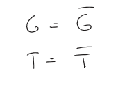
• We avoid discussion on how the government makes decisions regarding spending and taxes and just assume they are fixed (exogenously set variable means it is determined outside of the model and is treated as fixed or given.)

  Economists do not explain why it has that value inside the model; they simply assume it.

• Note: Fixed does not mean these values don’t change, it just means that their value is determined outside of the model.

Planned and Actual Expenditure

• Planned Aggregate Expenditure ($PE$): The total amount the economy plans to spend.

  • $PE = C + I + G$

• Actual Aggregate Expenditure ($AE$): The total amount the economy actually spends.

  • $AE = C + I_a + G$

  • This is physically how much people are buying.

• The Difference: The gap between $PE$ and $AE$ is the difference between planned and actual investment, which is the unplanned change in inventory.

  • If I_a > I, inventories are unexpectedly increasing.

  • If I_a < I, inventories are unexpectedly decreasing.

Market Equilibrium

• Definition: Equilibrium occurs when no one wants to change their decision; actual expenditure equals planned expenditure ($AE = PE$).

• Output and Expenditure: Since $AE$ is the expenditure approach to calculating GDP ($Y$), the equilibrium condition is:

  • $Y = PE$

• Adjustment Logic:

  1. If Y > PE (Aggregate Production > Planned Expenditure):

     • Firms produce more than is purchased.

     • Inventories unexpectedly accumulate (increase).

     • Firms respond by lowering production, thus reducing $Y$.

  2. If Y < PE (Aggregate Production < Planned Expenditure):

     • Firms produce less than is purchased.

     • Inventories unexpectedly fall (decrease).

     • Firms respond by increasing production, thus increasing $Y$.

Numerical and Graphical Equilibrium Example

• Model Equations:

  • $C = 100 + 0.5(Y - T)$

  • $I = 100 - 5r$

  • $G = 100$

  • $T = 50$

  • $r = 5$

• Numerical Calculation at $r = 5$:

  • $I = 100 - 5(5) = 75$

  • $PE = [100 + 0.5(Y - 50)] + 75 + 100$

  • $PE = 100 + 0.5Y - 25 + 75 + 100 = 250 + 0.5Y$

  • Set $Y = PE$: $Y = 250 + 0.5Y$

  • $0.5Y = 250 \rightarrow Y = 500$

• Graphical Equilibrium:

  • 45-degree Line: Represents points where $Y = PE$. This shows potential equilibria.

  • Planned Expenditure Line: In this case, $PE = 250 + 0.5Y$.

  • The intersection of these lines is the actual equilibrium ($Y = 500$).

Determinants of the Planned Expenditure ($PE$) Line

• Y-Intercept Changes:

  • Increase in Government Purchases ($G$): Increases intercept.

  • Increase in Interest Rate ($r$): Lowers investment, thus lowering intercept.

  • Increase in Taxes ($T$): Lowers intercept (due to impact on $C$).

• Slope Changes:

  • Marginal Propensity to Consume ($MPC$): Determines the slope. A larger $MPC$ results in a steeper $PE$ line.

The Investment Multiplier

• Scenario: Suppose the interest rate rises from $r = 5$ to $r = 10$.

  1. Original $I$ was $75$. New $I = 100 - 5(10) = 50$. Change in Investment ($\Delta I = -25$).

  2. New $PE$ equation: $PE = 100 + 0.5(Y - 50) + 50 + 100 = 225 + 0.5Y$.

  3. New Equilibrium: $Y = 225 + 0.5Y \rightarrow 0.5Y = 225 \rightarrow Y = 450$.

  4. Change in Output ($\Delta Y = 450 - 500 = -50$).

• Observation: Output fell by $50$, even though investment only fell by $25$. Output fell by more than the initial change in investment.

• Why does it fall by more? (The Multiplier Cycle):

  • Investment falls $\rightarrow PE$ falls $\rightarrow$ firms cut production $\rightarrow$ household income falls.

  • The fall in income causes consumption ($C$) to fall ($\Delta C = MPC \times \Delta Y$).

  • The fall in consumption further reduces $PE$, leading to more production cuts.

  • This cycle continues until a new equilibrium is reached.

• Multiplier Formula:

  • $\text{Multiplier} = \frac{\Delta Y}{\Delta I} = \frac{1}{1 - MPC}$

  • In the example: $MPC = 0.5$, so Multiplier $= \frac{1}{1 - 0.5} = 2$.

  • The total change: $\Delta Y = \text{Multiplier} \times \Delta I = 2 \times (-25) = -50$.

The IS Curve

• Definition: The IS curve represents the relationship between aggregate output ($Y$) and the interest rate ($r$) in the goods market.

• Relationship: There is a negative relationship between output and interest rates.

• Derivation Logic:

  1. If Interest Rate ($r$) increases $\rightarrow$ Investment ($I$) falls.

  2. Falling Investment ($I$) causes Planned Expenditure ($PE$) to fall.

  3. Falling $PE$ causes an unplanned increase in inventories.

  4. Firms respond by reducing production ($Y$).

  5. Therefore, higher $r$ corresponds to lower equilibrium $Y$.

• Sloping: The IS curve slopes downward because a higher interest rate reduces investment and planned expenditure, leading to lower equilibrium output.