MACHINE LEARNING final

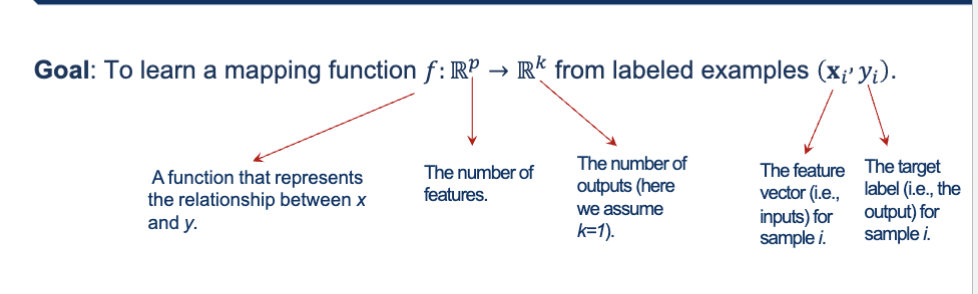
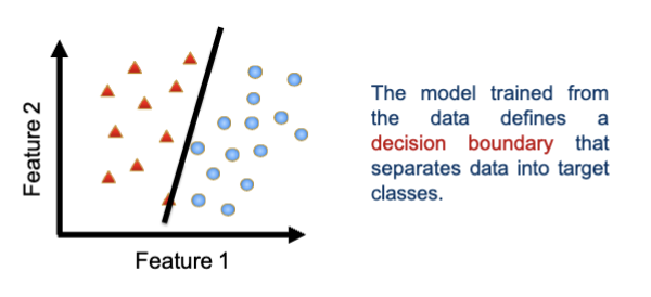
What is the goal of supervised learning?

To learn a mapping function f:R^p → R^k from labeled examples (xi,yi)

• You give the model examples → it learns a rule → it predicts outputs for new, unseen inputs.

What are the 2 types of supervised learning?

• Classification: predicts a categorical label

  • outputs are target classes/probablities (disease yes/no, email spam/no spam)

• Regression: predicts a continuous value

  • outputs are real values (temp, price)

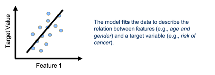
What is linear regression?

Goal: find the best straight line that predicts something

• prediction = (slope)(x+intercept)

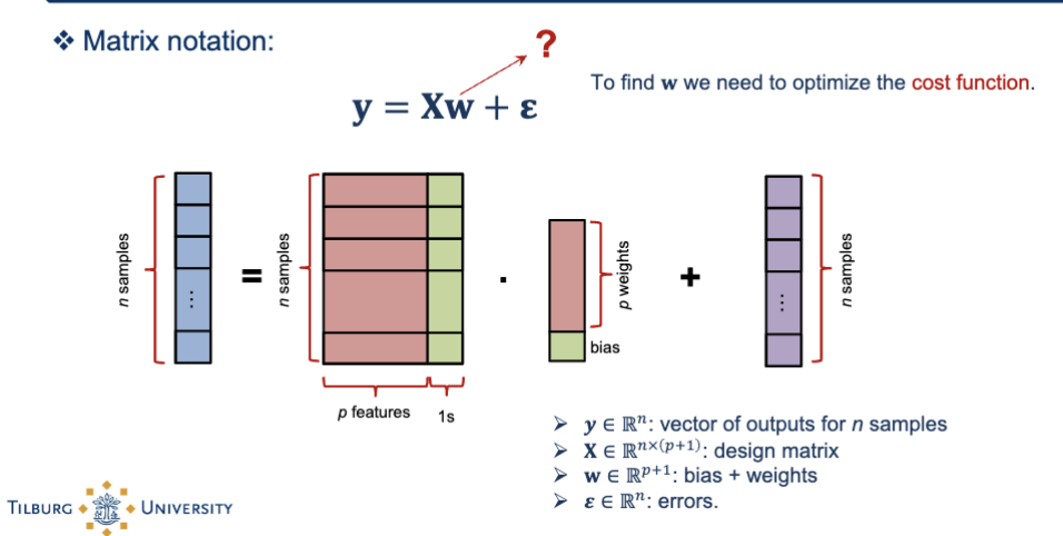
What is the matrix notation of linear regression?

y = Xw + e

• each row = one sample

• each column = one feature

• the first column is a column of ones (for the bias)

Prediction = weighted sum of features + bias

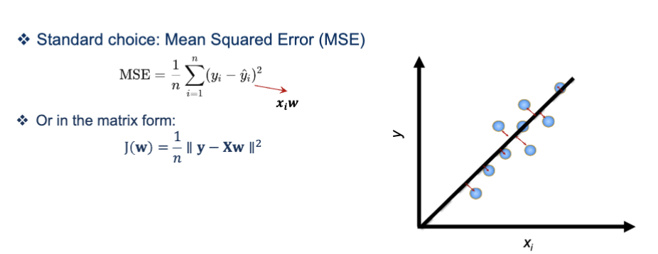
What is the connection between the cost function and linear regression?

by minizing the cost function, you find the best weights w for linear regression

• the matrix form measures how wrong the model is, smaller cost = better model

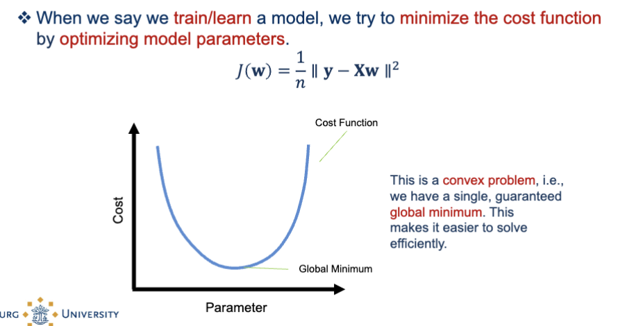
What is the convex problem in the cost function?

• The curve is shaped like a bowl

• There is one unique global minimum

• This minimum gives you the best possible weights

• No risk of getting stuck in a local minimum (unlike neural networks)

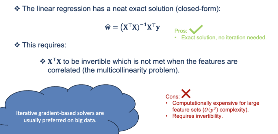
What is the neat exact solution of linear regression?

optimization - the analytical solution

• this is a formula that gives you the best weights w in one single calculation, without looping → called the normal equation

  • Instead of searching for the best line, this formula directly computes the best line.

When does it work?

Only when:

1. XTX is invertible, and

2. The number of features p is not huge.

If features are strongly correlated (e.g., height in cm and height in inches), you get multicollinearity, and XTX is not invertible.
→ Then you cannot use the formula.

✔ When shouldn’t you use the formula?

• If you have many features → matrix inverse is very slow

• If the design matrix is not invertible

So in real ML:

We rarely use the analytical solution.
Instead, we use gradient descent, which works even when the matrix isn’t invertible and when p is huge.

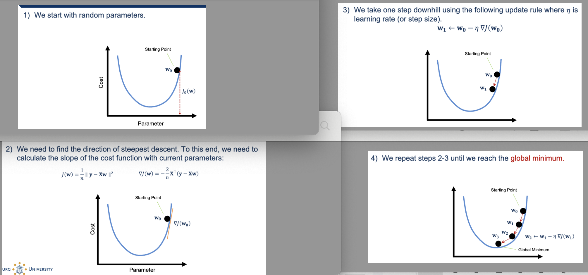
Describe the 4 steps of iterative optimization - gradient descent algorithm

1. start with random parameters

• start somewhere random on hill

• initial model w bad weights

2. We need to find the direction of steepest descent. To this end, we need to calculate the slope of the cost function with current parameters

3. We take one step downhill using the following update rule where 𝜂 is

learning rate (step size/amount you move)

• if learning rate is too big = overshooting, too small = move too slow

4. We repeat steps 2-3 until we reach the global minimum

• works for huge datasets, even when analytical solution is impossible

How can you estimate non-linear functions using linear regression?

Linear regression is only linear in the PARAMETERS (weights), not in the original features

What is feature engineering?

Transform the original input x into new features that capture non-linear patterns. Then run linear regression on those transformed features.

• Feature engineering = creating new, meaningful features from existing data so the model can learn patterns more easily.

• Feature engineering is the process of transforming your raw data into better inputs (features) that make your model perform much better.

🧠 Why do we need feature engineering?

Because many relationships in the real world are non-linear, messy, or hidden. Raw data often does NOT directly show the patterns we want the model to learn. Feature engineering helps us expose those patterns.

What are examples of feature engineering?

• polynomials: x²,x³

• interaction terms: x1x2

• logarithms: log(x)

• trigonometric functions: sin(x), cos(x)

• domain-specific features: ratios, counts

Linear Regression + Feature Engineering = very powerful model

• However, it can result in overfitting to training data.

• The relation between the complexity of the induced model and underfitting and overfitting is a crucial notion in data mining

feature engineering increases model complexity, more features = more flexibility = better ability to fit complicated patterns BUT higher risk of overfitting

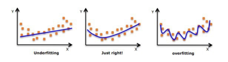
What is under and overfitting?

• underfitting: the induced model is not complex (flexible) enough to model data

  • too simple

  • predictions are bad on training and test data

• overfitting: the induced model is too complex (flexible) to model data and tries to fit noise

  • weights become very large

  • very good on training data but bad on test data

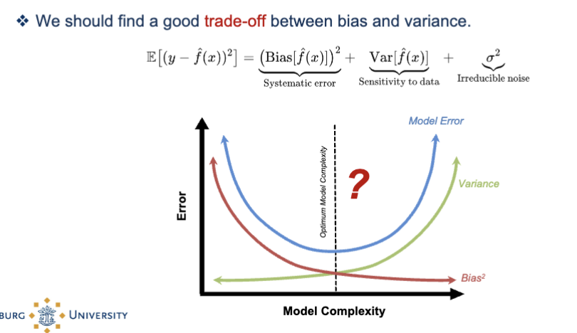
What is bias-variance trade-off?

Model error can be deconstructed into: bias² + variance + noise

• bias = error from being too simple (underfitting)

• variance = error from being too sensitive to training data (overfitting)

*high bias = too simple

*too complex = high variance

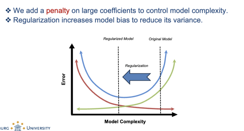
What is the solution to overfitting?

regularization

• shrinks weights to prevent overfitting

• Regularization = adding a penalty to the cost function to prevent the model from having huge coefficients → helps reduce overfitting and improves stability.

What regularization does:

• Adds a penalty on large coefficients

• This reduces variance

• But slightly increases bias

• Moves the model back toward the “just right” region in the bias–variance trade-off graph

👉 Underfitting is fixed by making the model more complex: add features, reduce regularization, or choose a more flexible model.

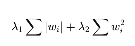
What are the 3 methods for regularization in linear regression?

1. Ridge (L2 penalization): Shrinks all coefficients smoothly

2. Lasso (L1 penalization): Encourages sparsity in coefficients

3. Elastic-net (L1+L2 penalization): Balances between ridge and Lasso

👉 A penalty is an extra cost added to the model when the weights become too large.

• large weights = overly complicated model = overfitting.

Method	Penalty	Effect	Best Use
Ridge	L2	Shrinks all coefficients smoothly	Multicollinearity, all features matter
Lasso	L1	Sets some coefficients exactly to zero	Feature selection, sparse models
Elastic Net	L1 + L2	Mix of sparsity + stability	Correlated features + many features

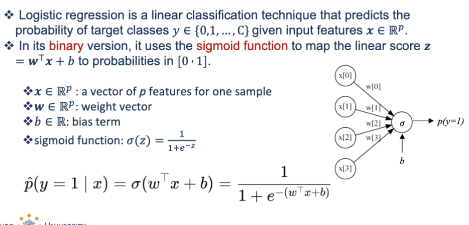
What is logistic regression?

• Logistic regression is a linear classifier.

• It predicts the probability of a class (in binary: 0 or 1).

• It uses input features x∈R^p

• The model has:

  • w = weight vector

  • b = bias

First computes a linear score: z = w^T x + b

Then applies the sigmoid function to convert z → probability:

• σ(z) = 1/ 1+e^-z