DATA MINING MIDTERM

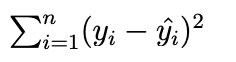
Sum of squared residuals

We estimate the linear regression coefficients by minimizing the _____

RSE( Residual squared error)

The standard deviation of the error and accuracy of the model is measured using ____

P-Value

The _____ can be used to reject the null hypothesis if < 0.05

MSE

The ____ is reported in units of Y

K-Nearest Neighbor

The _____ approach is a non-parametric method that makes a prediction based on the closest training observation

Cross validation (either LOOCV OR K-Fold)

Performing _____ ensures that every observation is selected for the testing data at least once

Decision Boundary (Discriminant function)

Linear discriminant analysis uses a _____ to seperate observations into distinct classes

Prior Probability

The ______ measures the probability that a random chosen observation belongs to class 

Posterior Probability

Refers to updated beliefs or probabilities after new data has been incorporated through Bayes' Theorem

Best Subset Selection

Performing ______ to sub-select predictors requires the user to check every possible combinations of predictors (2p).

Principal Component Analysis (PCA)

The ______ is unsupervised method used to transform the predictors (p) to a linear combination of the predictors (M, p ≥ M).

Knot

A _____ is a location where our coefficients and functions change.

Regression spline

The _______ is a combination of step functions and polynomial regression.

Random Forest

The Decision Tree based model can be improved upon by using bagging and sub-selecting predictors at each split, typically called _______.

Pure Nodes

The goal of splits in trees is to produce homogeneous child nodes, often called ______.

We can relax the additive assumption of linear regression by adding interaction terms.

True

Linear regression is applicable to datasets where p is larger than n.

False

Naive Bayes classifiers assumes that all predictors are independent within classes

True

Classifiers typically return a probability that a given observation belongs to class k.

True

It is expected that the training error rate is lower than the testing error rate.

True

A confusion matrix is used to assess accuracy for classification and regression models.

False

It is good practice to prevent data leakage by reusing the same sample in both training and testing.

False

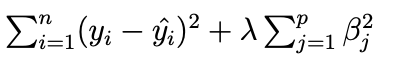
Both Ridge Regression and Lasso use a shrinkage penalty to regularize the coefficients to reduce the impact of the predictor on the model.

True

Forward and Backward Stepwise Selection are guaranteed to find the best possible combinations of predictors.

False

Cross Validation is often the best method to find the most optimal parameters.

True

Basis Functions are fixed, known functions (bk(X)) that transform X to allow us to use statistical tools like Standard Errors and Coefficient estimates.

True

For splines, it is best practice to use fewer knots to increase flexibility in regions where it may be necessary.

False

Generalized Additive Models allow us to use more than one predictor in our model.

True

Ridge Regression

Smoothing Splines

Linear Regression

Lasso Regression

Linear Regression

Logistic Regression

Ridge Regression

Polynomial Regression

Step Functions

Lasso Regression

Regression Splines

Tree Based Models

Non-Linear

Classification and Regression Trees (CART) (Decision Trees)

Goal of the decision tree is to split the data into like chunks or pure nodes

Then use the tree structure to make inferences on data

Makes few assumptions about the input dataset

○ No linearity assumptions!

Graph Theory

Gini of Split

Used to split decision tree chunks

Want the split with the lowest possible Gini Impurity

If multiple are equal randomly choose one

Get for all predictors

How do we know to stop splitting?

Tree Depth - how many times do you want to split the data?

Minimum samples in leaf - how small do you want the leaf nodes?

Feature Importance

Tells us how much each input variable (feature) contributes to the prediction of a model

It helps us understand which features matter most in determining the output

Decision Tree Split Types

Classification - Gini, Entropy, Log Lost

Regression - MSE, Absolute Error, Poisson

Cost Complexity Pruning (Weakest Link Pruning)

A very large tree may overfit the data, want to prune the tree by removing some of the unnecessary branches

Start at full deep tree with many terminal nodes (𝛼=0), as 𝛼 increases the cost of having so many terminal nodes increases, and branches get pruned

Cross Validation to find optimal 𝛼, but 𝛼 and T are interacting so often people use them interchangeably

Improvement on Decision Trees

Decision Trees are weak learners with high variance

• Eachs split will be very different from each other

• We can use Decision Trees as the base for more complex models

Bootstrapping

Sub select the samples for the root node at random

Sampling without replacement, can be selected only once

Out of Bag (OOB) Error Estimation

Average the error across trees

Is a valid estimate of the test data since none of the individual trees have seen the given test sample

Random Forest (RF)

Sub-select the samples for the root node at random (using bootstrapping)

Sub-select the features at random at each split (sampling without replacement, can be selected only once)

Trees within the forest are not pruned

Boosted Trees

Builds trees sequentially

For each data point, calculate the difference between the predicted value and the actual value.

These residuals represent what the first tree did not predict correctly.

• This way, it focuses on the mistakes of the previous tree.

Fits each tree hard and may overfit, Boosted Trees are a slow learner

Fit each tree to the residuals of the previous tree instead of Ytrain

Iterative Random Forest (iRF)

The model is retrained multiple times, giving more weight to features that were consistently important in previous iterations.

This helps stabilize the identification of truly important features and reduce noise.

Basis Functions

Very simple extensions of linear models

• Polynomial Regression

• Step Functions (Piecewise-Constant Regression)

• Splines

Basis functions b1 (X), b2 (X), … , bK (X) are fixed, known, and hand selected

• Transforming X into something else

• Like Linear Regression, all of the statistical tools are applicable here too

  • Standard Errors

  • Coefficient estimates

  • F-statistics

Polynomial Regression

The standard way to extend linear and logistic regression

• Add polynomial terms (X d )

  • Typically d ≤ 4

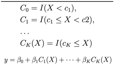
Step Functions

• Uses step functions to avoid imposing a global structure

• Break X into bins, turn into ordered categorical variables/dummy variables

• Good for variables that have natural break points

  • Ex: 5 year age bins

  • Are poor predictors at the breakpoints

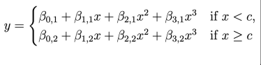
Regression Splines

• Type of basis function that is a combination of polynomial regression and step functions

• Locations where the coefficients/functions change are called knots

  • More knots, more flexible method

• Adding a constraint removes a degree of freedom, reducing complexity! (smoothing it out)

Natural Splines

• Splines can have high variance at the outer range of X

• Natural spline - adds boundary constraints, must be linear at the boundaries

  • Boundaries - the region smaller than the smallest K and the region larger than the largest K

Smoothing Splines

• Different approach, still produces a spline

• Places a knot at every value of X

• Uses penalty to determine smoothness

• λ is the smoothing parameter controlling the trade-off:

  • Small λ≈0\lambda \approx 0λ≈0 → very flexible, almost interpolates data → high variance.

  • Large λ→∞\lambda \to \inftyλ→∞ → heavily penalizes wiggles → approaches a straight line → low variance, high bias.

Local Regression

• Instead of fitting one global regression to all the data, this fits a regression only around the target point x0

• Nearby observations have more influence on the fit at x0​, while distant points have little or no effect.

• Conceptually, this is similar to K-nearest neighbors (KNN), except:

  • KNN predicts by averaging nearby y-values.

  • Local regression predicts by fitting a weighted regression locally.

Generalized Additive Models (GAMs)

• The model is additive:

  • The effect of each predictor is added together.

  • There are no interaction terms by default.

• This keeps the model interpretable:

  • You can examine how each variable individually affects the response.

• Allow you to use splines, natural splines, smoothing splines, or local regression for each predictor.

• The only restriction: the contributions of predictors are added together, not multiplied or combined in complex ways (unless you specifically include interaction terms)

Subset Selection

Reducing the number of predictors by selecting a subset of the predictors and evaluating the performance of that subset compared to other subsets of predictors

Best Subset Selection

• This model predicts the sample mean for each observation.
  Try combinations of predictors to find the one with the smallest RSS or largest R squared

• Total of 2p possible models, computational intensive

• If p is large (high dimensional data), may suffer from statistical problems for some models

Forward Stepwise Selection

• Test all predictors seperately

• Find the best predictor and tack on other predictors

• Only adds predictors that are improving the model

• Not guaranteed to find best possible combinations of predictors

• Can be used in high dimensional data (n < p) with special considerations (Do not pass Mn-1)

Backward Stepwise Selection

• Start with the full model (all predictors included).

• Iteratively remove the least useful predictor (based on some criterion) one at a time.

• Stop when removing more predictors would make the model worse.

• Select the single best model using highest p-value (prediction error)

• AIC BIC or R2

• If p is large (high dimensional data), may suffer from statistical problems for some model

How to choose the best model?

Can measure this error:

• Indirectly - by adjusting training accuracy measurements

• Directly - by using a test/validation set, or KFold/LOO cross validation approach

• Prediction focus? → CpC_pCp​ or AIC.

• Simplicity & interpretability? → BIC.

• Regression only, intuitive? → Adjusted R2R^2R2

Cp​ Statistic

• Adds a penalty to training RSS

• Penalizes models with more predictors

• Lower CpC_pCp​ → better model.

Akaike Information Criterion (AIC)

• Adds penalty, only defined for models fit by maximum likelihood

• Lower AIC is better

• Works when models are fit by maximum likelihood (e.g., regression, logistic regression)

Bayesian Information Criterion (BIC)

• Heavier penalty when nnn is large.

• Tends to select simpler models than AIC

Adjusted R 2

• Essentially, a perfect fit would have only correct variables and no noise

• Unlike plain R2, adding useless predictors decreases adjusted R2R^2R2.

• Higher adjusted R2 → better model

Direct Measurement of Test Error

• Report on the test/holdout/validation set of observations 

• Perform a cross validation (either LOO or KFold)

• Advantages over indirect measurement, makes fewer assumptions about the true model

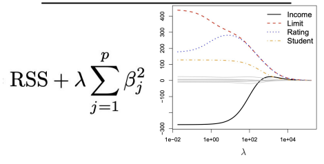
Shrinkage Methods

• Aim to “shrink” or regularize the coefficients so that they are essentially equal to zero

• Reduces the effect of the predictor on the model

Ridge Regression

• As 𝜆 →∞, shrinkage penalty increases, shrinks coefficient close to 0, is only equal to zero when 𝜆 = ∞

• All regression lines get close to 0 at the same time

• Will always use all the predictors (but some may have small coefficients)

• Does not use Beta 0

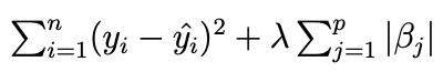
Lasso

• coefficient estimates not only shrink to zero, some may be equal to zero and removed from the model entirely (variable selection)

• Regression lines hit 0 at different times

• Can use only a subset of the predictors (variable selection)

Which Shrinkage Method?

In general, ridge regression might be better if all of the predictors are contributing to the response at least a little bit, lasso may be better if certain that some predictors are equal to zero

Dimension Reduction

Here we will transform the predictors

Principal Component Analysis

• Reduce number of predictors from p to M, by performing mathematical transformations to the existing predictors

• Transform the original correlated features into a set of uncorrelated variables, called principal components

• Adding any Zs will be automatically perpendicular or orthagonal to the last Z

• Unsupervised

Principal Components Regression

• When predictors X1,X2,…,XpX_1, X_2, \dots, X_pX1​,X2​,…,Xp​ are highly correlated, standard linear regression can become unstable.

• Reduces the predictors to a smaller set of uncorrelated principal components (PCs) and then uses them as inputs for regression.

• Doesn’t use the original predictors directly; it uses the top MMM components (usually the ones explaining most variance) as inputs for the regression.

• Assumes that the principal components capturing most variance in Xare also the ones that matter for predicting Y

• does use Y when computing ZM , is supervised

Classification

Assigns class info each sample (qualitative, categorical)

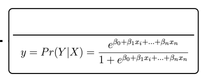
Logistic Regression

Models the probability that Y belongs to a particular category

Maximum Likelihood Estimation

Selecting 𝛽0 and 𝛽1 such that the predicted probability of (default = yes) is as close as possible the individual’s observed default status

Multinomial Logistic Regression

Allows for K > 2

Assumes that the odds for one class does not depend on the other

Predictors do not necessarily need to be explicitly independent, however low correlation between variables is preferred

K - 1

Runs idependent binary models

• Banana vs Apple → binary model

• Cherry vs Apple → binary model

Generative Models

If classes are too far apart

If X is approximately normal in each class and the sample size is small, generative models can be more accurate

Easier to extend to more than two response classes

Bayes Theorem

πk​=P(Y=k) = probability that a randomly chosen observation belongs to class K.

• Example:

  • πApple=05→ 50% of all fruits are Apples.

  • πBanana=0.3→ 30% Bananas.

  • πCherry​=0.2 → 20% Cherries.

Linear Discriminant Analysis

• Prior probability = your initial belief about a class.

• Likelihood = how well the observed data fits that class.

• Posterior probability = updated belief after seeing the data.

• For each observation, calculate the discriminant for each class, assign to the class with the highest discriminant

• To find the LDA decision boundary, find the point where these two discriminants are equivalent

• Performs best with fewer observations, reducing the variance is important

Quadratic Discriminant Analysis

Like LDA, with the difference of a class specific variance rather an a common variance (how far they differ from the mean), allows for quadratic shaped decision boundaries

Performs best with large amounts of observations

Naive Bayes Classifier

Does not combine predictors in each class, but assumes they are independent

If Xj is quantitative:

○ Can assume within each class, the j th predictor comes from a normal distribution

In a line up of apples count every 5th apple as data

K-Nearest Neighbors

• Non parametric

• Many observations

• Select a value of K, plot all training observations, for each test observation find the K nearest training observations, assign predicted value to test observation based on average known response value for the K nearest training observations

Generalized Linear Models

Useful when data is neither qualitative nor quantitative

○ Value more closely represents counts of a unit

○ Ex: CaBi ride share data, predicting number of riders

LDA & Logistic Regression

• When it can be linear

• Yes/No situation

QDA and Naive Bayes

• Moderately non-linear boundaries

• QDA allows each class to have its own covariance (curved boundaries).

• Naive Bayes can capture more complex shapes depending on predictor distributions.

Non-parametric approach like KNN

• Very non-linear boundaries

• KNN does not assume any formula for the boundary. It decides based on local neighborhoods.

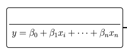
Linear Regression

• Predicts a quantitative response

• Assumes a linear relationship between predictor variables and the response variable

Parametric method

Estimate the parameters by minimizing the residual

𝛽0

Intercept

Starting point of the line

Unknown and Estimated

𝛽1

Slope

Unkown and estimated

Simple Linear Regression

Predicts a quantitative (numeric) response Y using a single predictor (independent variable) X

^

Indicates predicted value