CP421 Data Mining Week 8

Give the purpose of recommendations and when they became necessary

When we have a large catalogue of items (e.g., products of Amazon, movies of Netflix), users can interact with it in 2 ways:

• User knows what they’re looking for, and they search for that item

• Often, users don’t know exactly what they’re looking for. This is where recommendations come in. The system suggests items based on what they know about the user.

  • Recommendations became necessary when we moved from an era of scarcity to abundance (e.g., shelf space is a scarce commodity for traditional stores like Walmart and thus items were scarce, but nowadays sites on the web like Amazon enable an abundance of items to be presented at once). Thus, with more choices, we need better filters and recommendations.

Explain the three types of recommendations

1. editorial and hand curated (e.g., list of favourites, list of essential items)

2. simple aggregates (e.g., top 10, most popular, recent uploads)

3. tailored to individual users (Amazon, Netflix, etc.)

Provide the formal model for producing ratings for items

X = set of customers

S = set of items

Utility function u: X * S → R (i.e., u takes any customer+item pair and maps it to a rating)

• R = totally ordered set of ratings (e.g., 0-5 stars)

The results of u can be placed in a utility matrix U

• row i = customer i

• column j = item j

• cell i,j = customer i’s rating for item j

Are all cell values typically filled in a utility matrix U? How does this relate to the goal of recommendation systems?

A utility matrix is generally sparse (i.e., many values are not filled in since most customer can’t/won’t rate every item). The key goal of recommendation systems is to figure out these unknown values based on the known values (and, in turn, recommend highly rated items).

What are the 3 key problems to tackle when dealing with recommendation systems?

1. Gathering “known” ratings in the utility matrix (i.e., how to collect)

2. Extrapolating unknown ratings from the known ones

   • here, we’re mainly interested in high unknown ratings (i.e., knowing what you’ll like), since that’s what the system will recommend

3. Evaluating extrapolation methods

   • once we have a recommendation system that extrapolates unknown ratings from known ratings, how do we measure the success/performance of recommendations?

What are the 2 ways to gather known ratings?

1. Explicit: ask people to rate items

   • doesn’t work well in practice since people can’t be bothered (i.e., it doesn’t scale because only a small fraction of users leave ratings)

   • thus, great data but not sufficient in size

2. Implicit: learn ratings from user actions

   • e.g., purchase implies high rating

   • more scalable approach, but it’s difficult to learn low ratings (although it’s easy to learn high ratings)

In practice, most recommendation systems use a combination of both approaches.

What are the 3 ways to extrapolate unknown ratings from known ones? Mention the 2 key problems as well.

One key problem with extrapolating is that the utility matrix U is sparse (since most people have not rated most items).  This introduces many problems.

Another problem is that we often have a cold start (new items have no ratings, new users have no history).

There are three approaches we can take to extrapolate unknown ratings:

1. content-based

2. collaborative

3. latent factor based

Explain (in detail) how content-based recommendation systems work

Main idea: recommend items to customer x that are similar to previous items they rated highly (e.g., recommend movies with the same actors, director, genre, etc.)

It works as follows:

1. create an item profile i (i.e., feature vector) for each item

   • e.g., if items = movies, then an item’s profile may be a boolean vector [Actor 1, Actor 2, Actor 3, Director 1, Director 2, …], where a value of 1 means that actor or director participated in that movie

2. build a user profile x using the profiles of items they’ve rated (i₁,…,i_n); this can be a weighted average of rated item profiles (where each item’s weight = user’s rating), or a normalized weighted average using (user’s rating for item - user’s average rating) as weights

   • x=[x₁,…,x_k], where each x_i=weighted average of feature i; ultimately, x represents each user based on the items they like

   • e.g., USER PROFILE = UNWEIGHTED MEAN OF ITEM PROFILES: assume items = movies, and item profile = boolean vector for each actor (i.e., each actor represents one feature). Suppose user x has watched 5 movies, where 2/5 movies feature actor A, and 3/5 movies feature actor B. Then, user x’s profile is the mean of item profiles, where feature A’s profile weight is 2/5 and feature B’s profile weight is 3/5.
     x = mean of 5 item profiles = [2/5, 3/5, …]

   • e.g., USER PROFILE = NORMALIZED WEIGHTED MEAN OF ITEM PROFILES USING RATINGS: now, assume actor A’s movies are rated 3 and 5, while actor B’s movies are rated 1, 2, and 4. Then, assuming the user’s mean rating is 3, we can normalize each actor’s ratings (by doing (user’s rating - average rating): actor A’s normalized ratings now become 0 and +2, and the profile weight for this feature becomes (0+2)/2=1. Similarly, actor B’s normalized ratings become -2, -1, 1, and the profile weight for this feature becomes (-2-1+1)/3=-2/3. This indicates a mild positive preference for actor A and a mild negative preference for actor B.
     NOTE: when calculating each feature’s profile weight here, we divide by # items with that feature, not by total # items like above
     x = [1, -2/3, …]

3. given user profile x and a new item’s profile i, we can assign it a similarity score:
   u(x,i) = cos(x,i) = (dot(x,i))/(mag(x) * mag(i))
   ^^ we recommend items with the highest cosine similarity: close to 1 = item contains features the user likes, close to -1 = item contains features the user tends to dislike, close to 0 = neutral preference

NOTE: mag(A) = sqrt(a1² + a2² + … + an²)

Give the 4 pros of the content-based approach

1. no need for data on other users

2. able to recommend to users with unique tastes (unlike collaborative filtering, which relies on the existence of similar users)

3. able to recommend new and unpopular items (i.e., no first-rater problem, since an item is recommended purely based on its profile (regardless of its ratings))

4. we can provide explanations for recommended items (e.g., user x was recommended item i because of feature k)

Give the 3 cons of the content-based approach

1. Finding the appropriate features is hard (i.e., which features should we use to appropriately represent movies, images, music, etc.?)

   • this is the main reason why this approach isn’t as popular

2. Overspecialization: this approach never recommends items outside the user’s content profile, which causes issues when users have multiple interests/preferences but only expressed some of them in the past. Additionally, this approach is unable to exploit high-quality judgements of other users (e.g., if many users have rated a movie extremely highly, a user who never expressed interest in that type of movie will never have it recommended to them).

3. Cold-start problem for new users: how do we build a user profile if the user hasn’t rated any items?

Explain the general structure of collaborative filtering

Given a user x, we find a set N of other users whose ratings are “similar” to x’s ratings. Then, we estimate x’s ratings based on ratings of users in N (i.e., we see items that users in N prefer, and recommend those items to user x)

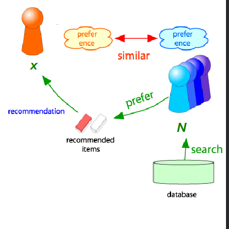
how does a similarity metric work in general, and what are the 3 types?

sim(x,y) = similarity metric between users x and y (with rating vectors r_x and r_y)

1. Jaccard similarity

2. Cosine similarity

3. Centered cosine similarity

Explain how Jaccard similarity works, and how we’d calculate sim(A,B) and sim(A,C) here. Mention the key problem with it.

Recall, rA and rB are the rating vectors for users A and B

Sim(A,B) = |rA n rB| / |rA u rB|

i.e., (number of items both A and B have rated) / (number of items either A or B have rated)

So, sim(A,B) = 1/5, and sim(A,C)=2/4. Therefore A is more similar to C than B.

However, a key issue with this approach is that it IGNORES actual rating values. This is why we incorrectly predicted that A is more similar to C than B; in theory, A should be more similar to B.

Explain how Cosine similarity works, and how we’d calculate sim(A,B) and sim(A,C) here. Mention the key problem with it.

Sim(A,B) = cos(rA, rB) = dot(rA, rB) / (mag(rA) * mag(rB))

So, sim(A,B) = 0.38, and sim(A,C) = 0.32. Therefore A is (correctly) more similar to B than C, but not by much.

Key issue: this approach treats a missing rating as negative.

NOTE: for a vector 𝑣⃗=(3,4), it’s magnitude is sqrt(3²+4²) = sqrt(25) = 5

Explain how Centered Cosine similarity works, and how we’d calculate sim(A,B) and sim(A,C) here. Mention why this approach is best compared to others.

First, we normalize ratings by subtracting the row mean.

Then, using these new values, we calculate:

sim(A,B) = cos(rA, rB) = dot(rA, rB) / (mag(rA) * mag(rB))

So, sim(A, B) = 0.09 and sim(A, C) = -0.56. Therefore A is (correctly) more similar to B than C.

This method captures intuition better than base cosine similarity since missing ratings are treated as “average” and it handles “tough rates” and “easy” rates.

This method is also known as Pearson Correlation.

for collaborative filtering, how do we go from similarity metric to recommendations?

i.e., once we have similar users to user x, how do we use them to predict user x’s rating of item i?

Let r_x be the vector of user x’s ratings, and let N be the set of k users most similar to x who have rated item i. 

Then, the prediction of user x’s rating of item i:

r_xi = [sum for all yEN] (dot(s_xy,r_yi)) / [sum for all yEN] (s_xy)

where s_xy = sim(x,y)

and r_yi = user y’s rating of item i

How do we perform item-item collaborative filtering? i.e., what’s the procedure for rating an item i based on similar items?

so far, we’ve covered user-user collaborative filtering, but another view is item-item collaborative filtering.

steps:

1. find similar items to item i

2. estimate rating for item i based on ratings for similar items:

r_xi = [sum for all jEN(i;x)] (dot(s_ij, r_xj)) / [sum for all jEN(i;x)] (s_ij)

where

N(i;x) = set of items rated by x that are similar to item i,

s_ij = similarity of items i and j,

r_xj = user u’s rating of item j

what’s better, item-item collaborative filtering, or user-user?

In practice, it has been observed that item-item collaborative filtering often works better than user-user.

Why? Because items are simpler, and users have multiple tastes.

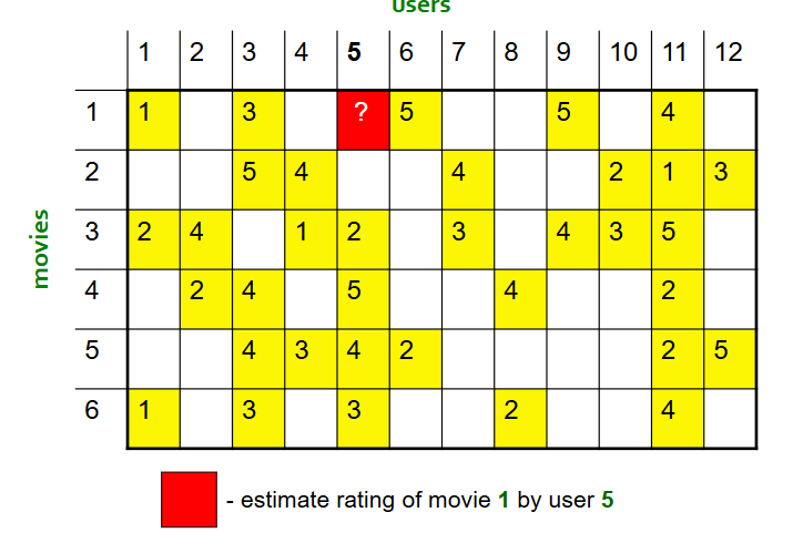
using this matrix, use item-item collaborative filtering to estimate user 5’s rating of movie 1.

1. compute pearson correlation between movie 1 and all other movies:

   • subtract each movie’s mean rating

   • treat each row (movie as a vector)

   • compute cosine similarity between these normalized vectors

result:

sim(1,1) = similarity weight/score between movie 1 and movie 1 = 1

sim(1,2) = -0.18

sim(1,3) = 0.41

sim(1,4) = -0.10

sim(1,5) = -0.31

sim(1,6) = 0.59

2. identify all movies that are (1) similar to movie 1, and (2) rated by user 5. User 5 has only rated movies 3, 4, 5, and 6. Of those movies, only movies 3 and 6 have a positive similarity score, therefore these are the only similar movies, and we select these moving forward.

   1. remember, sim(x,y) > 0 means movies are similar and attract similar users, = 0 means movies have no detectable relationship, and < 0 means movies are dissimilar and attract opposite audiences (i.e., users that like movie x tend to dislike movie y, and vice versa)

3. take s_1,3 = 0.41 and s_1,6 = 0.59, which are the similarity weights between movies 1 and 6 and movies 3 and 6.

4. compute r_ix = user x’s estimated rating of item i = [sum through all items (j) rated by user x that are similar to i] (dot(s_ij, r_jx)) / [sum through all items (j) rated by user x that are similar to i] (s_ij)
   = (0.41 × 2 + 0.59 × 3) / (0.41 + 0.59) = 2.6
   therefore, user x’s estimated rating of item i is 2.6.

Final interpretation: user 5 has never rated movie 1, but they have rated movie 6 = 3 (which is very similar to movie 1) and movie 3 = 2 (which is moderately similar to movie 1). So, the system gives more weight to movie 6 and concludes that user 5 will probably rate movie 1 around 2.6 stars.

What’s the main advantage of collaborative filtering?

It works for any kind of item, since no feature selection is needed (i.e., items don’t need to be represented by features)

what are the 4 disadvantages of collaborative filtering?

1. cold start: we need enough users in the system to find a match

2. sparsity: the user/ratings matrix is sparse, and it’s hard to find users that have rated the same items

3. first rater: we cannot recommend an item that hasn’t been previously rates (thus new items struggle)

4. popularity bias: we cannot recommend items to someone with unique taste (i.e., the system tends to recommend popular items)

what are the 2 hybrid methods we can use for recommendation systems?

1. add content-based methods to collaborative filtering

   • item profiles for the new item problem

   • demographics to deal with the new user problem

2. implement two or more different recommenders and combine predictions

   • perhaps using a linear model

   • e.g., global baseline + collaborative filtering

     • global baseline: estimate Joe’s rating for movie M. However, assume Joe has not rated any movie “similar” to movie M. So the global baseline approach is as follows:

       • mean movie rating = 3.7 stars

       • movie M is rated 0.5 stars above average

       • joe rates 0.2 stars below average

       • therefore, baseline estimate is 3.7 + 0.5 - 0.2 = 4 stars

     • local neighborhood (collaborative filtering): Joe didn’t like related movie N, and rated it 1 star below his average rating

     • final estimate: Joe will rate movie M 4-1=3 stars

what are the 3 levels of recommender systems?

A modern recommender system performs multi-scale modeling of the data:

1. Global: overall deviations of users/movies

   • e.g., mean movie rating on Netflix: 3.7 stars, movie x is rated 0.5 stars above average, Joe rates 0.2 stars below average, therefore baseline estimation is that Joe rates movie x 3.7+0.5-0.2=4 stars

2. Factorization: addressing “regional” effects

3. Collaborative filtering: extracting local patterns (i.e., local neighbourhood)

   • e.g., Joe didn’t like related movie y, so the final estimate is that Joe will rate movie x 3.8 stars

NOTE: RMSE of global models > RMSE of collaborative filtering models > RMSE of latent factor models

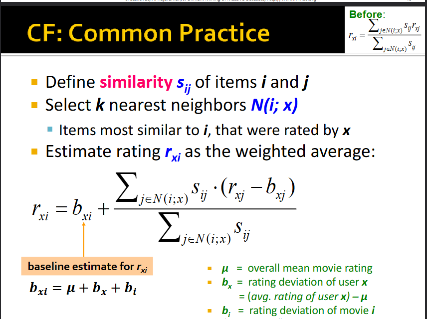
Explain how we combine collaborative filtering with baseline estimates

see pic

e.g., mean movie rating on Netflix: 3.7 stars, movie x is rated 0.5 stars above average, Joe rates 0.2 stars below average, therefore baseline estimation is that Joe rates movie x 3.7-0.2+0.5=4 stars.

In this example, mu = 3.7, bx = 0.2, and bi = 0.5

jEN(i;x) → iterate through the j most similar items to i

Sij → similarity between items i and j

rxj → user x’s rating of item j

bxj → baseline estimate of user x’s rating for item j (overall mean + (user x’s average rating - overall mean) + (item j’s average rating - overall mean)

Thus, first part (bxi) is the global part of the model and the second part is the collaborative filtering part of the model.

How do we evaluate the effectiveness of a recommender system using the item/user ratings matrix (i.e., utility matrix)?

1. remove a chunk of ratings from the sparse item/user ratings matrix (perhaps the bottom right quadrant); store these ratings in the test set (T)

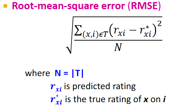
2. make predictions, and compare your predictions with the known ratings in the test set (T) using the formula in the pic (RMSE)

RMSE explanation:

1. store the sum of (predicted rating - actual rating)² for each user/item pair in the test set

2. divide the sum by the size of the test set (i.e., number of user/item pairs in the test set)

3. take the square root of the result

NOTE: RMSE is the most commonly used measure to evaluate a collaborative filtering system

what’s the goal of latent factor model recommendation systems?

Goal: make good recommendations

• we quantify goodness using RMSE: lower RMSE = better recommendations

  • RMSE = root mean square error; if RMSE is 0.95, this means the estimated rating is 0.95 stars away from the true rating

• even though we want to make good recommendations on items the user hasn’t seen yet, this isn’t possible

• so, instead, we build a system that works well in predicting hidden known (user, item) ratings, and hope the system will also work well in predicting truly unknown ratings

i.e., we’re thinking of recommendations as an optimization problem (an ML approach)

How do Latent Factor Models work in terms of singular value decomposition?

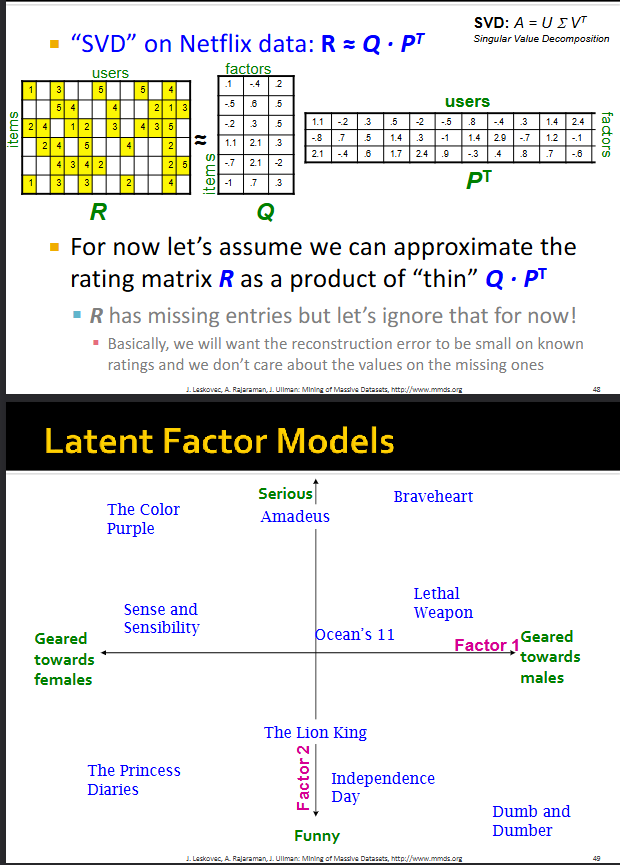
This method relies on matrix factorization (i.e., factorizing the item/user utility matrix).

We apply a version of singular value decomposition (SVD) to the utility matrix as follows:

• Given utility matrix R, we try to represent it as a product of two matrices Q and P: R = Q * P^t

  • Q and P are “thin” and “long” matrices, where Q has one row per item with k columns (factors) and P^t has one column per user with k rows (factors)

  • k is a parameter we choose; it’s usually less than the total number of users

• Now, this means each item and user is represented as a data point in the same k-dimensional space. e.g., item i is represented by the k values in the i’th row of matrix Q, while user j is represented by the k values in the j’th column of matrix P^t

  • the axes of this k-dimensional space (i.e., “axes of variation”) are the “factors”

• Ultimately, Latent Factor Recommendation Models find a lower-dimensional representations of items and users, where items and users that are close together represent good recommendations

NOTE: in the pic, for some reason, we represent the items/users in a 2D space even though we have k=3 factors in the slide before

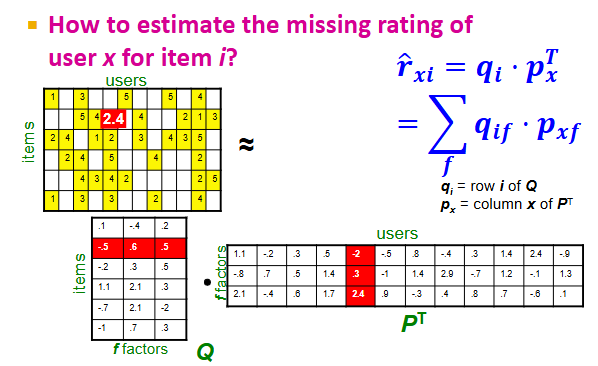
In Latent Factor Recommendation Systems, how do we estimate the missing rating of user x for item i (i.e., cell i, x in utility matrix R)?

Recall, we represented the utility matrix R as Q * P^t

To estimate the value on the i’th row and x’th column of R (i.e., user x’s rating of item i), we compute the following:

r_xi = dot(q_i, p_x^t) = dot((row i of Q), (column x of P^t))

In plain English, this rating estimate looks at how close the user and item are located in the k-dimensional factor space (closer = better)

In Latent Factor Recommendation Systems, how do we determine optimal Q and P (i.e., how do we find the latent factors)?

Recall, we represented the utility matrix R as Q * P^t

Background: SVD uses the minimized sum of squared errors to determine optimal P and Q. However, SVD goes through ALL values in the utility matrix R, and isn’t defined when entries are missing; no rating is interpreted as zero rating. In our case, R is often sparse and has missing entries. So, we need another approach to find P and Q.

Approach: minimize RMSE on training data (i.e., find P and Q such that predicted ratings are as close to the true ratings as possible), hoping that it also minimizes RMSE on unseen test data:

• f(P, Q) = [sum for all (i,x)ER] (r_xi - dot(q_i, p_x^t))² 

  • NOTE: here, we’re only iterating through the values of matrix R that are in the training set; we’re not iterating through any values in the test set (bottom right quadrant of R)

• find P and Q that minimize f via gradient descent:

  • compute derivative f’

  • start at some point y and evaluate f’(y); this gives us the gradient (slope) of f at y

  • take a step in the reverse direction of the gradient: y = y - f’(y)

  • repeat re-computations of y until converged

• for this problem specifically, gradient descent looks like this:

  • initialize P and Q (using SVD, pretend missing ratings are 0)

  • perform gradient descent for P and Q:

    • P ← P - n*P’

      • P’ = derivative of matrix P, which is just the derivative of the function f(P, Q) we’re minimizing with respect to p_x = [sum for all (i,x)ER] (-2 * q_ik (r_xi - dot(q_i, p_x^t)))

      • n = learning rate

    • Q ← Q - n*Q’

      • Q’ = derivative of f(P, Q) with respect to q_i = [sum for all (i,x)ER] (-2 * p_xk (r_xi - dot(q_i, p_x^t)))

    • repeat re-computations of P and Q until convergence

For Latent Factor Recommendation models, explain the need for regularization and how we implement it

When finding the latent factors, we’re minimizing RMSE on training data. The goal is to find k (# factors) that is large enough to capture all signals. However, RMSE on the test set begins to rise for k > 2 (i.e., larger k = larger test error).

This is an example of overfitting. With too much freedom (too many free parameters via large k), the model starts fitting noise. This means the model performs well on the training data but fails to generalize well on unseen test data.

Solution: modify optimization function using regularization, allowing for a rich model where there is sufficient data but shrinking aggresively where data is scarce.

• min(P,Q) = error + lambda*length

• error = RMSE of training data (what we’ve used before)

  • we want this to be small

• lambda = non-negative value set by you; balances tradeoff between model complexity and training error (closer to 0 = model complexity is irrelevant and error is prioritized, closer to infinity = model complexity is prioritized and simpler model is produced)

• length = number of factors describing each user

  • if the user has rated many items, we tolerate a larger length (i.e., we wouldn’t want to make the user’s latent factors too short, so we tolerate more complex factors for that user)

  • if the user hasn’t rated many items, we want the length to be small (i.e., we want the distance of the user to the origin in the k-dimensional space to be small)