CI 460 Machine Learning

ERAU

Irreducible Error

inherent noise or variability in the data that cannot be reduced.

Reducible Error

Error that can be reduced by improving the model

Prediction

estimation, we can make accurate predictions for the response

Inference

(inference) if we can understand how the output changes based on the input

Parametric Methods

Assume the functional form of F, fixed number of parameters. Simple with less flexibility. Examples: linear regression, logistic regression

Non-parametric methods

Learns directly from the data, adapts to complex patterns. Needs more training data and are more flexible. Examples: decision trees, random forests, KNN

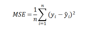
MSE (Mean Squared Error)

Measure used to asses quality of fit/accuracy for regression model. Always want to minimize MSE.

MSE

Squared difference between actual and predicted values

• n - number of observations

• yi - observed values

• ^yi - predicted values

MSE example

• True Y = [14, 7, 5, 9]

• Predicted Y = [4, 8, 8, 10]

• MSE = ( (14- 4)^2 + (7 - 8)^2 + (5 - 8)^2 + (9-10)^2 ) / 8

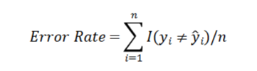
Error Rate

Measuring Quality of fit for classification. If the condition gives a 1 then the condition is incorrect, otherwise is a zero. Error rate represents a fraction of the incorrect classifications.

Loss Function

Measures how far the prediction is from the true outcome and assigns a numerical penalty to the incorrect predictions. Want to choose the weights that minimize the loss.

• EX - MSE, Error Rate

Bias

(underfitting) error from modeling problems with too simple of the model. (Using a linear model to try and fit a complex pattern)

Variance

(Overfitting) How much the output (f) would change based on a different training data set. More flexible the model the more variance

Bias Variance Trade off

The more flexible the model the higher the variance and the less bias

Bayes Error Rate

Irreducible error in classification. It is the lowest error rate that any classifier can achieve.

KNN (K Nearest Neighbors)

Classification, Regression, uses the closest neighbors to decide classification, Non-parametric.

• K = small value → High variance and low bias

• In higher dimensions performs worse and fits to the noise

• Is sensitive to scaling

Scaling

• Scaling - making sure that no one feature will dominate the distance and outcome, pre processing technique

• algorithms that have gradient decent need scaling

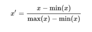
Normalization

when doesn’t linear conclusion

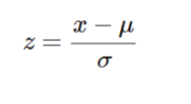
Standardization

when data follows a normal distribution

Peaking Phenomenon

As features go up so does performance until optimal and then goes down as more and more features are added.

Curse of Dimensionality

When the dimension is so high that all the points are basically the same distance apart and the center of the cube is empty. Need to reduce features

Binary Classifier Evaluation

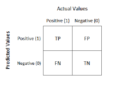
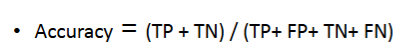
Accuracy

Sensitivity

True Positive Rate

TP/ ( TP +FN )

Specificity

Specificity is the proportion of actual negatives that got predicted

True Negative Rate

TN / ( TN + FP)

1 - Specificity

False Positive Rate

FP / ( FP + TN)

Logit Output

Probability Output

P( y=1 | x)

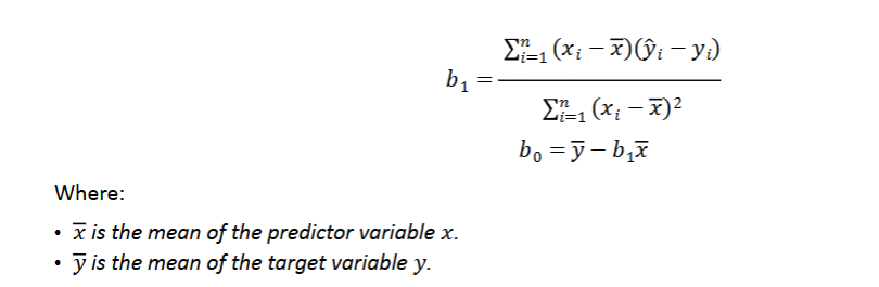
OLS (Ordinary Least Squared)

Minimizes the squared differences between actual and predicted values

Uses MSE and the Residuals

Normal Equations

• Closed form solution

• Minimize MSE

• For simple linear regression, smaller datasets, and for model parameters

Gradient Decent

• Efficient for large datasets and high dimensions

• scales well in machine learning

• iterative optimization algorithm to minimize the loss function

Normal Equations

• Closed form solution

• efficient for smaller datasets with few features

Precision

TP / ( TP + FP )

Information Theory

Study of qualification, storage, and digital information

• Founded by Harry Nyquist, Ralph Hartley, Claude Shannon

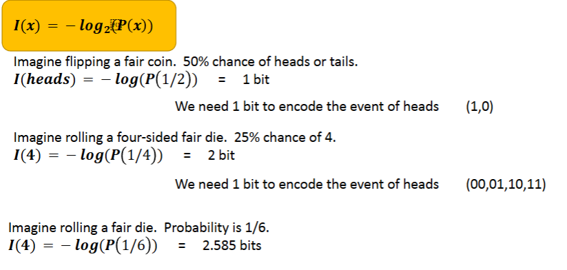
Quantifying Information

• Low probability event → high information (surprising)

• High probability event → low information

Self Information

The measure of the information associated with the outcome of a random variable, (How much information is in a given variable)

• 1 unit of information = 1 bit

• I(x) = -log(P(x))

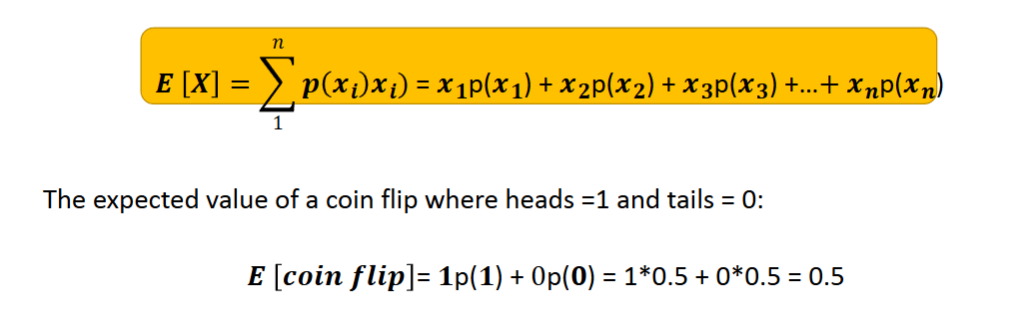
Expected Value

The long term average

Entropy

The measure of the average uncertainty associated with a given random variable

Self Information vs Entropy

• Self Information → measures the information/uncertainty in an event

• Entropy → the amount of uncertainty/information in a set of events

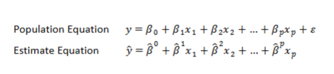
Linear Regression

• Models the relationship between the dependent and independent variable by using line of best fit

Gradient decent is efficient for

large datasets and high dimensions, scales well

least squares fit in terns of linear regression

is used to minimize the differences between the predicted and actual values.

normal equations are good for

small datasets and small features, involve inverting a matrix

Regression sum of squares

SST = SSR + SSE

• SSTotal - total squared distance of observations of mean of y

• SSRegression - distance from regression line to mean of y

• SSRedidual (SSE) - variance around the regression line that is not explained by the regression line (this is what we are trying to minimize)

Coefficient of Determination (R²)

• values range from 0 - 1

• 0 - model does not explain any variability in the data

• 1 - the model perfectly explains the variability in the data

• R² = SSR/SST

• The Higher the R² the better fit of the model to the data

Logistic Regression

for classification problems

instead of predicting y we predict P(Y=1) (aka yes or no)

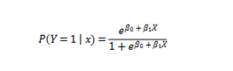
Logistic regression gives an

s shaped curve

odds ratio

measure that gives the change in the odds of an outcome if everything else is constant

• values close to 0 indicate very low or very high probabilites

Logit

ROC vs AUC

• ROC measures the classifier performance over all thresholds

• AUC (area under the roc curve) - single numbered score that summarizes the performance

Regression Trees

• Regression problems

• divide predictor space into distinct regions

Split regression trees by using

the results with the lowest mse or entropy in the training data

Classification tree

• predictions are categorical not continuous (regression)

• split by minimizing the error rate

we know how far back to prune a tree by

using cross validation to see which tree has the lowest error rate

CP

Complexity parameter, use to control complexity and accuracy trade off

Pros vs Cons of decision trees

• Pro - Trees are easy to explain, plotted graphically, used for both classification and regression

• Cons - Don’t have prediction accuracy as more complicated models

Bagging

• bootstrap aggregating

  • resampling of the observed dataset done by random sampling with replacement from the og dataset

  • averaging reduces variance

  • gives lots of training datasets

  • less interpretation

In random forests variable importance is computed

Through mean decrease gini

Mean Decrease Gini vs Entropy

• Both used to evaluate quality of split

• Gini - Based on probability of missclassification

• Entropy - based on the amount of information needed to identify the class of an element

Random Forests

• Same process as bagging but de-correlates the trees

• Done by taking a random sample of predictors every time a split is considered

When random forests are built using m = p

This amounts to being a bagged tree

Validation Set Approach

• Split data into training and testing (validation)

• build multiple models and test on lowest error rate

• can be highly variable

Leave - one - out cross validation

• split data of size n into

  • training - n-1

  • test (validation) 1

• validate and find mse

• Has less bias, variability, computationally intensive

K - fold cross validation

• divide dataset into parts

• remove one part and test on last part

• repeat with different part each time

• average k different mse’s

• more accurate, balances bias/variance trade off for error estimates